

Siimulation of Tandem Cylinders Using OpenFoam and LibAcoustics Library


Simulation of tandem cylinders in OpenFOAM using the libAcoustics library
Note:
- This tutorial has only didactic purpose, aiming to help beginners, and it does not guarantee quality of simulation results. Verification and validation of the results, and also the study of mesh refinement and other analyzes are left as responsibility of the user.
- This offering is not approved or endorsed by OpenCFD Limited, producer and distributor of the OpenFOAM software via www.openfoam.com, and owner of the OPENFOAM® and OpenCFD® trade marks.
- This tutorial was created within the context of an UFSC extension project and it is not approved by LibAcoustics and OpenFOAM® developers.
- OpenFOAM version 1912 was used.
- This tutorial was prepared by the undegraduate students Julio Victor Viera, under the supervision of Filipe Dutra da Silva.
- Please quote this page if you use this material. Questions and suggestions can be sent to the contact addresses shown at the end of this page.
In this tutorial will be presented the steps for simulating a tandem cylinder case in OpenFOAM together with the libAcoustics library created by Epikhin et al., using a 3D dipole case. This library contains the implementation of acoustic analogies that allow the calculation of noise in far-field from aerodynamic data collected close to the source. First, the acoustic pressure in the time domain is calculated. Then, these data are converted to the frequency domain using the Fast Fourier Transform (FFT) algorithm. Here we will make use of the Ffowcs Williams-Hawkings (FWH) analogy and the Curle analogy.
Note: Before installing the libAcoustics library, you must have installed the FFTW library.
Vamos utilizar como base um caso do próprio OpenFOAM e também um caso da biblioteca de acústica. Vá até o local onde o OpenFOAM está instalado e abra o seguinte diretório: tutorials/incompressible/pisoFoam/RAS. Copie a pasta “cavity” e cole onde você deseja salvar o tutorial com o nome “tutorialCilindros”.
Let’s use a case from OpenFOAM itself and also a case from the acoustics library as a basis. Go to the location where OpenFOAM is installed and open the following directory: tutorials/incompressible/pisoFoam/RAS. Copy the “cavity” folder and paste where you want to save the tutorial with the name “tutorialCilindros”.
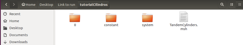
The first step is to import the mesh previously generated in Gmsh (See tutorial). To do this, copy the file “TandemCylinders.msh” and paste it inside the “tutorialCilindros” folder. So the following files should be seen inside the folder like this:
Delete the “system” folder, because we are going to use a model of a case from the acoustic library. Then, open the “Tutorials” folder that is together with the libAcoustics library installation files (not to be confused with the OpenFOAM “tutorials” folder). Open the “dipole3D” case, copy the “system” folder and paste it into the “tutorialCilindros” folder.
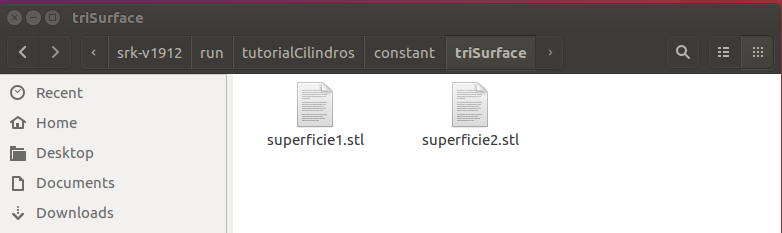
Open the “constant” folder and inside it create a folder named “triSurface”. Now copy the surfaces generated in Gmsh (“superficie1.stl” and “superficie2.stl”) and paste it inside the “triSurface” folder.
Next, open the terminal and go to the folder of the case. Type “gmshToFoam TandemCylinders.msh” and press “enter”. This command converts the format of the Gmsh mesh to the format used in OpenFOAM.

Now, type “checkMesh” at the terminal and press “enter”. If everything is ok with the mesh, the message “Mesh OK” should appear.

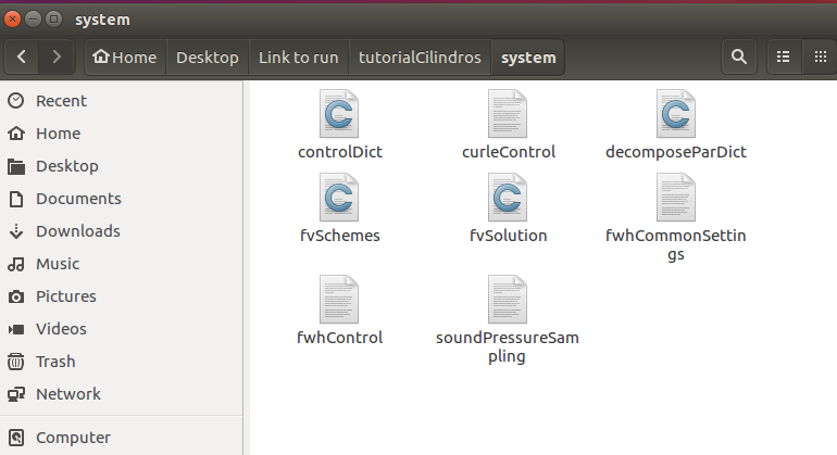
The next step is to edit the files of the copied model for the cylinder case settings. Inside the “tutorialCilindros” folder, open the “system” folder. The files that will be used are shown below. The other files can be deleted.
Then, open the “controlDict” file. Let’s use the “pisoFoam” solver. Make all modifications according to the settings shown below:
application pisoFoam;
 startFrom latestTime;
 startTime 0;
 stopAt endTime;
 endTime 0.2;
 deltaT 0.25e-4;
 writeControl timeStep;
 writeInterval 1000;
 purgeWrite 0;
 writeFormat ascii;
 writePrecision 6;
 writeCompression on;
 timeFormat general;
 timePrecision 6;
 runTimeModifiable true;
 adjustTimeStep false;
 maxCo 2;
 maxDeltaT 1e-3;

 functions
 {
    #include "curleControl"
    #include "fwhControl"
    #include "soundPressureSampling"
 }
Note: in “functions” are inserted the functions of the aeroacoustics library.
Done the necessary changes, save the “controlDict” file and close it.
Still inside the “system” folder, open the “fvSchemes” file. The following numerical schemes will be used (the other schemes that appear in the model must be deleted):
ddtSchemes
 {
      default backward;
 }

d2dt2Schemes
 {
      default Euler;
 }

gradSchemes
 {
      default Gauss linear;
      grad(p) Gauss linear;
      grad(U) Gauss linear;
 }
 divSchemes
 {
      default Gauss limitedLinear 1;
      div((nuEff*dev2(T(grad(U))))) Gauss linear;
 }
 laplacianSchemes
 {
      default Gauss linear corrected;
 }
 interpolationSchemes
 {
      default linear;
      interpolate(U) linear;
 }
 snGradSchemes
 {
      default corrected;
 }
 fluxRequired
 {
      default no;
      p ;
      pcorr ;

 }
 wallDist
 {
       method meshWave;
 }
Save the “fvSchemes” file and close it.
Now, open the “fvSolution” file. Let’s use the following settings:
solvers
{
p
{
 solver PCG;
 tolerance 1e-07;
 relTol 1e-3;
 preconditioner
 {
 preconditioner GAMG;
 tolerance 1e-5;
 relTol 0.01;
 smoother GaussSeidel;
 nPreSweeps 0;
 nPostSweeps 2;
 cacheAgglomeration no;
 nCellsInCoarsestLevel 100;
 agglomerator faceAreaPair;
 mergeLevels 1;
 }

}

pFinal
{
    $p;
    relTol 1e-6;
}
"(U|k|omega)"
{
    solver          smoothSolver;
    smoother        DILUGaussSeidel;
    tolerance       1e-08;
    relTol          0;
}
 } PISO
  {
  nOuterCorrectors 1;
  nCorrectors 3;
  nNonOrthogonalCorrectors 1;
  pRefCell 0;
  pRefValue 0;
  momentumPredictor true;
  }
Save the changes made and close the file.
Open the “decomposeParDict” file. In “numberOfSubdomains” change the value to the number of processors you want to use on your machine to run the simulation in parallel. Save the change and close the file.
Now, open the “curleControl” file. In it, the settings of the Curle analogy will be defined. It must be configured as follows:
CurleAnalogy
 {
 libs (“libAcoustics.so”);
 type Curle;
 log true;
 probeFrequency 1;
 patches (cyl-1 cyl-2);
 timeStart 0.16;
 timeEnd 0.2;
 c0 343;
 dRef -1;
 pName p;
 pInf 0;
 rho rhoInf;
 rhoInf 1.225;
 CofR (0 0 0);
 writeFft true;
 U0 (44 0 0);

observers
{
    microphone-A
    {
    position    (-0.4761 1.5896 0.4572);
    pRef        2.0e-5;
    fftFreq        1024;
    }
    microphone-B
    {
    position    (0.5206 1.8288 0.457);
    pRef        2.0e-5;
    fftFreq        1024;
    }
    microphone-C
    {
    position    (1.5173 1.5896 0.457);
    pRef        2.0e-5;
    fftFreq        1024;
    }
}
 }
In “patches” are specified the surfaces on which the input data for the Curle analogy will be stored, which in this case are the surfaces of the two cylinders. To skip the transient regime, we start the analogy at just 0.16 seconds. The “c0” indicates the speed of propagation of sound in the air. The “dRef” refers to the domain thickness for 2D simulations, but as this case is 3D, we ignore this function by changing its value to a negative number. Finally, we have in “observers” the points in the far field where the noise levels will be measured. The “fftFreq” indicates the amount of data present in a window in which the FFT is applied.
After making the changes, save and close the “curleControl” file.
Then open the “fwhCommonSettings” file to define the FWH analogy settings. Let’s use definitions similar to the Curle analogy. To do this, replace the contents of the file with the following below:
libs ("libAcoustics.so");

log             true;
writeFft        true;
probeFrequency  1;
timeStart       0.16;
timeEnd         0.2;
c0              343;
dRef            -1;
pName        p;
pInf            0;
rho             rhoInf;
rhoInf          1.225;
CofR            (0 0 0);
U0            (44 0 0);

observers
{
    microphone-A
    {
    position    (-0.4761 1.5896 0.4572);
    pRef        2.0e-5;
    fftFreq        1024;
    }
    microphone-B
    {
    position    (0.5206 1.8288 0.457);
    pRef        2.0e-5;
    fftFreq        1024;
    }
    microphone-C
    {
    position    (1.5173 1.5896 0.457);
    pRef        2.0e-5;
    fftFreq        1024;
    }
}
Save the “fwhCommonSettings” file and close it.
Now, open the “fwhControl” file. For the Curle analogy, the surfaces used for data acquisition are the cylinder surfaces themselves (defined in “patches” in the “curleControl” file). As for the FWH analogy, the surfaces to be used are those generated in Gmsh in the format .stl and inserted in the /constant/triSurface folder. The settings for these surfaces are defined in the “fwhControl” file. Replace your content with the following:
superficie1
 {
 type FfowcsWilliamsHawkings;

#include            "fwhCommonSettings";
patches             (cyl-1 cyl-2);
formulationType     GTFormulation;
cleanFreq           100;

interpolationScheme insideCells;

surfaces
(
    superficie1
    {
        type            sampledTriSurfaceMesh;
        surface         superficie1.stl;
        source          insideCells;
        interpolate     false;
    }

);

     nonUniformSurfaceMotion false;
     Ufwh                    (0 0.0 0.0);

     fixedResponseDelay  true;
     responseDelay       1e-6;
}
superficie2
{
  type FfowcsWilliamsHawkings;
  #include            "fwhCommonSettings";
  patches             (cyl-1 cyl-2);
  formulationType     GTFormulation;
  cleanFreq           100;

  interpolationScheme insideCells;

  surfaces
  (
    superficie2
    {
        type            sampledTriSurfaceMesh;
        surface         superficie2.stl;
        source          insideCells;
        interpolate     false;
    }

  );

  nonUniformSurfaceMotion false;
  Ufwh                    (0.0 0.0 0.0);

  fixedResponseDelay  true;
  responseDelay       1e-6;
 }
The acquisition surfaces in “surfaces” are those inside the “triSurface” folder and not the surfaces of the cylinders. The “Ufwh” is used when a mobile surface is desired, but in this case we will use stationary surfaces.
Once the changes are made, save the “fwhControl” file and close it.
The last file belonging to the library is “soundPressureSampling”. Open it and replace its contents with the one shown below. In there, the data that the surfaces must collect are configured and also the way in which they must be saved.
surfacePressure{type soundPressureSampler;libs (“libAcoustics.so”);writeControl timeStep;writeInterval 1;outputGeometryFormat gmsh; fields ( p ); pName p; log true; interpolationScheme cellPoint; surfaces ( superficie1 { type sampledTriSurfaceMesh; surface superficie1.stl; source cells; interpolate true; } superficie2 { type sampledTriSurfaceMesh; surface superficie2.stl; source cells; interpolate true; } );}
After applying the changes, save and close the file.
The settings of the files in the “system” folder are complete. Go back to the “tutorialCilindros” directory and open the “constant” folder and then open the “transportProperties” file. In it, enter the viscosity and density of the air as shown below.
transportModel Newtonian;nu nu [ 0 2 -1 0 0 0 0 ] 1.47e-05;
rho rho [ 1 -3 0 0 0 0 0 ] 1.225;
rho [ 1 -3 0 0 0 0 0 ] 1.225;Still in the “constant” folder, open the “turbulenceProperties” file. The turbulence model to be used is the “kOmegaSST”.
simulationType RAS;
RAS{
RASModel kOmegaSST;
turbulence on;
printCoeffs on;
}Save the changes and close the file.
Go to the “polyMesh” folder and open the “boundary” file. Let’s change the face type of the two cylinders to wall. To do this, change the “type” and “physicalType” from “patch” to “wall” on both cylinders. The other settings remain unchanged, as shown below.
6
(
frontAndBack
{
type patch;
physicalType patch;
nFaces 39536;
startFace 569932;
}
free
{
type patch;
physicalType patch;
nFaces 3320;
startFace 609468;
}
inlet
{
type patch;
physicalType patch;
nFaces 1120;
startFace 612788;
}
outlet
{
type patch;
physicalType patch;
nFaces 1120;
startFace 613908;
}
cyl-1
{
type wall;
physicalType wall;
nFaces 560;
startFace 615028;
}
cyl-2
{
type wall;
physicalType wall;
nFaces 560;
startFace 615588;
}
Save the “boundary” file and close it. Return to the “tutorialCilindros” directory.
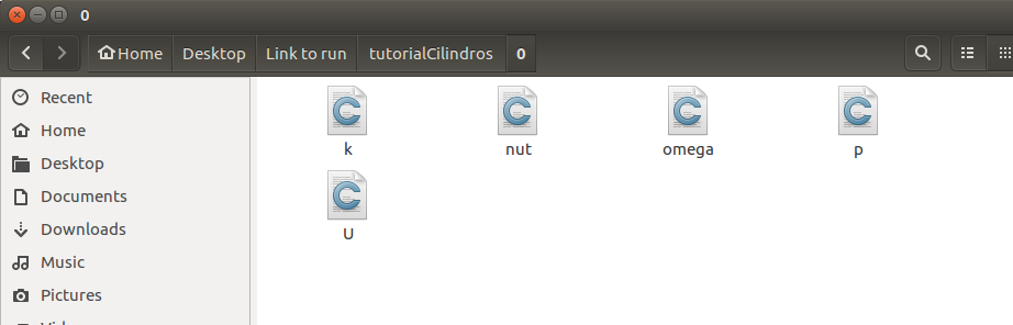
Finally, let’s define the boundary conditions. Open the “0” folder. The “epsilon” and “nuTilda” files must be deleted, leaving only the files shown below.
Replace the contents of each file as shown below.
“k” :
dimensions [0 2 -2 0 0 0 0];
internalField uniform 0.00325;
boundaryField
{
inlet
{
type freestream;
freestreamValue $internalField;
}
outlet
{
type zeroGradient;
}
cyl-1
{
type kqRWallFunction;
value uniform 0.00325;
}
cyl-2
{
type kqRWallFunction;
value uniform 0.00325;
}
free
{
type freestream;
freestreamValue $internalField;
}
frontAndBack
{
type zeroGradient;
}
}
“nut” :
dimensions [0 2 -1 0 0 0 0];
internalField uniform 0;
boundaryField
{
inlet
{
type calculated;
value uniform 0;
}
outlet
{
type calculated;
value uniform 0;
}
cyl-1
{
type nutUSpaldingWallFunction;
value uniform 0;
}
cyl-2
{
type nutUSpaldingWallFunction;
value uniform 0;
}
free
{
type calculated;
value uniform 0;
}
frontAndBack
{
type zeroGradient;
}
}“omega” :
dimensions [0 0 -1 0 0 0 0];
internalField uniform 43;
boundaryField
{
inlet
{
type freestream;
freestreamValue $internalField;
}
outlet
{
type zeroGradient;
}
cyl-1
{
type omegaWallFunction;
value $internalField;
}
cyl-2
{
type omegaWallFunction;
value $internalField;
}
free
{
type freestream;
freestreamValue $internalField;
}
frontAndBack
{
type zeroGradient;
}
Note: we use wall function on cylinders for each of the above files.
“p” :
dimensions [0 2 -2 0 0 0 0];
internalField uniform 0;
boundaryField
{
inlet
{
type freestreamPressure;
freestreamValue uniform 0;
}
outlet
{
type fixedValue;
value uniform 0;
}
cyl-1
{
type zeroGradient;
}
cyl-2
{
type zeroGradient;
}
free
{
type freestreamPressure;
freestreamValue uniform 0;
}
frontAndBack
{
type zeroGradient;
}
}“U” :
dimensions [0 1 -1 0 0 0 0];internalField uniform (44 0 0);
boundaryField
{
inlet
{
type freestreamVelocity;
freestreamValue uniform (44 0 0);
}
outlet
{
type zeroGradient;
}
cyl-1
{
type noSlip;
}
cyl-2
{
type noSlip;
}
free
{
type freestreamVelocity;
freestreamValue uniform (44 0 0);
}
frontAndBack
{
type slip;
}
}Obs: Para a pressão na entrada utilizamos a pressão de corrente livre. Para a velocidade, utilizamos a condição de não escorregamento em ambos os cilindros.
Note: For the inlet pressure we use the free current pressure. For speed, we use the no-slip condition on both cylinders.
Now, we can start the simulation. Open the terminal and go to the “tutorialCilindros” case directory. First, let’s decompose the domain to run in parallel. Type “decomposePar” no terminal.

Then, type “mpirun -np 5 pisoFoam -parallel > log &” to run the simulation (replace the number 5 with the number of processors configured in the “decomposeParDict” file).

Note: The simulation may take a few hours. The details of the process are being recorded in the “log” file inside the “tutorialCilindros” folder.
Post processing
Finished the simulation, type “reconstructPar -latestTime” in terminal to get the last step of the simulation.

To check the value of y+, type “pisoFoam -postProcess -func yPlus”.

Before opening the results in Paraview, it is necessary to create a file with the .foam extension. To do this, type “nano cilindros.foam” and press “enter”. Then press “ctrl + o”, “enter” and finally “ctrl + x”.

To open Paraview, type “paraview cilindros.foam”

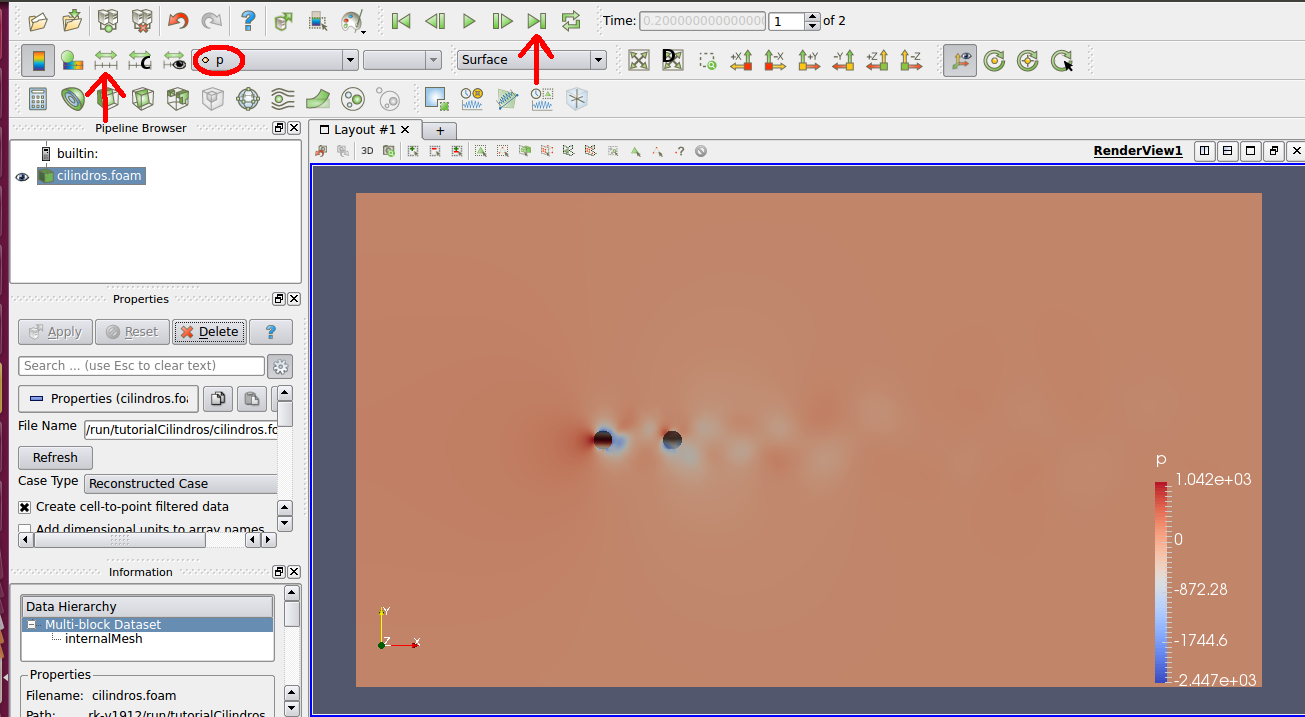
In Paraview, click Apply. To view the pressure field, first select the last time step and also click on the option “Rescale to data range” as shown in the figure below.
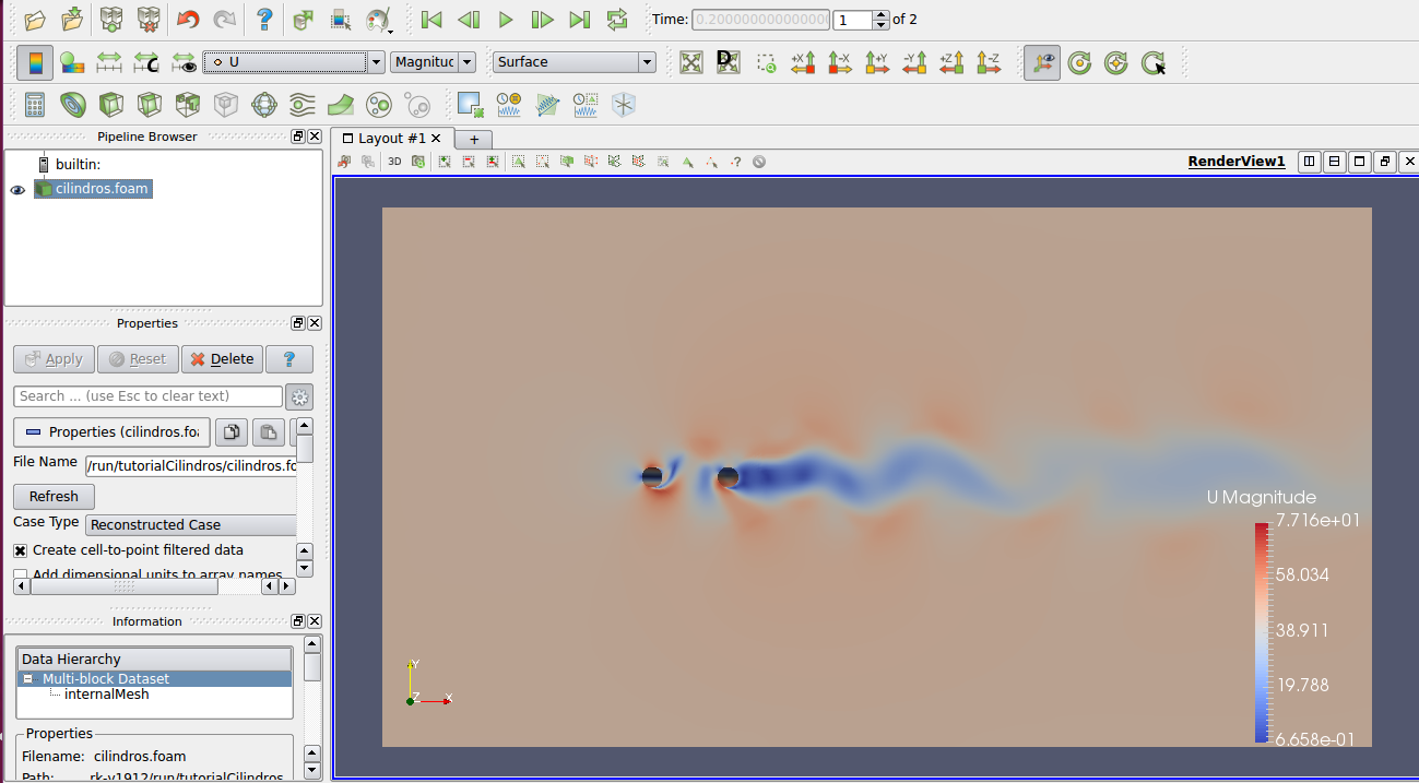
The velocity field has the following result:
The acoustic data can be found in the “acousticData” folder inside the “tutorialCilindros” folder. To plot the graphs related to the acoustic data, a code in Matlab will be used here.
First, you need to import the data. With Matlab open, go to the “Home” tab and click on “ImportData”. Go to the directory “tutorialCilindros” and open the “acousticData” folder. Let’s plot the results for microphone A. Then select the file “fftCurleAnalogymicrophoneA” and click on “Open”. In the window that opens, click on the “ImportSelection” option. Repeat the same procedure to open the files “fft-surface1-microphone-A” and “fft-surface2-microphone-A”.
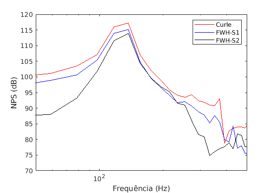
To plot the comparative graph between the three results, that is, using the FWH analogy with surfaces 1 and 2, and also using the Curle analogy, the following code is executed:
% Frequências
fCurle = fftCurleAnalogymicrophoneA{:,1};
fS1 = fftsuperficie1microphoneA{:,1};
fS2 = fftsuperficie2microphoneA{:,1};
% Nível de Pressão Sonora
splCurle = fftCurleAnalogymicrophoneA{:,3};
splS1 = fftsuperficie1microphoneA{:,3};
splS2 = fftsuperficie2microphoneA{:,3};
% Espectro de frequência
semilogx(fCurle,splCurle,’-r’)
hold on
semilogx(fS1,splS1,’-b’)
hold on
semilogx(fS2,splS2,’-k’)
hold on
xlabel(“Frequência (Hz)”)
ylabel(“NPS (dB)”)
xlim([50 500])
legend(“Curle”, “FWH-S1”, “FWH-S2”)
Thus, the result obtained is:
Note: For better results, you can increase the number of points per FFT block (nfft), both in the “fwhCommonSettings” file and in the “curleControl” file. However, by increasing the nfft it may also be necessary to increase the simulation time. It is also worth mentioning that the mesh used has merely didactic purposes and that if the objective is to obtain results close to experimental values, refinements in the simulation model must be applied.


