

Mesh Generation Tutorial of Tandem Cylinders Using Gmsh


Mesh Generation Tutorial of Tandem Cylinders Using Gmsh
Note:
- This tutorial has only didactic purpose, aiming to help beginners, and it does not guarantee quality of simulation results. Verification and validation of the results, and also the study of mesh refinement and other analyzes are left as responsibility of the user.
- This offering is not approved or endorsed by OpenCFD Limited, producer and distributor of the OpenFOAM software via www.openfoam.com, and owner of the OPENFOAM® and OpenCFD® trade marks.
- This tutorial was created within the context of an UFSC extension project and it is not approved by GMSH and OpenFOAM® developers.
- This tutorial was prepared by the undegraduate students Julio Victor Viera and Widmark Kauê Silva Cardoso under the supervision of Filipe Dutra da Silva
- Please quote this page if you use this material. Questions and suggestions can be sent to the contact addresses shown at the end of this page.
This tutorial presents the procedures for generating a structured mesh of tandem cylinders using Gmsh. Both the steps to generate the mesh through the graphical interface and the script will be presented.
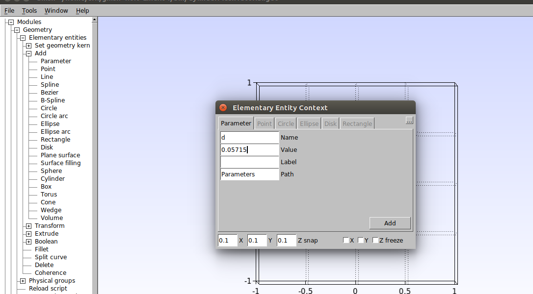
First, let’s define the parameters that will be useful throughout the process. With Gmsh open click on Modules→Geometry→Elementary Entities → Add → Parameter. . In the window that opens, set the cylinder diameter value as 0.05715 and click on “Add”, as shown in the figure below.
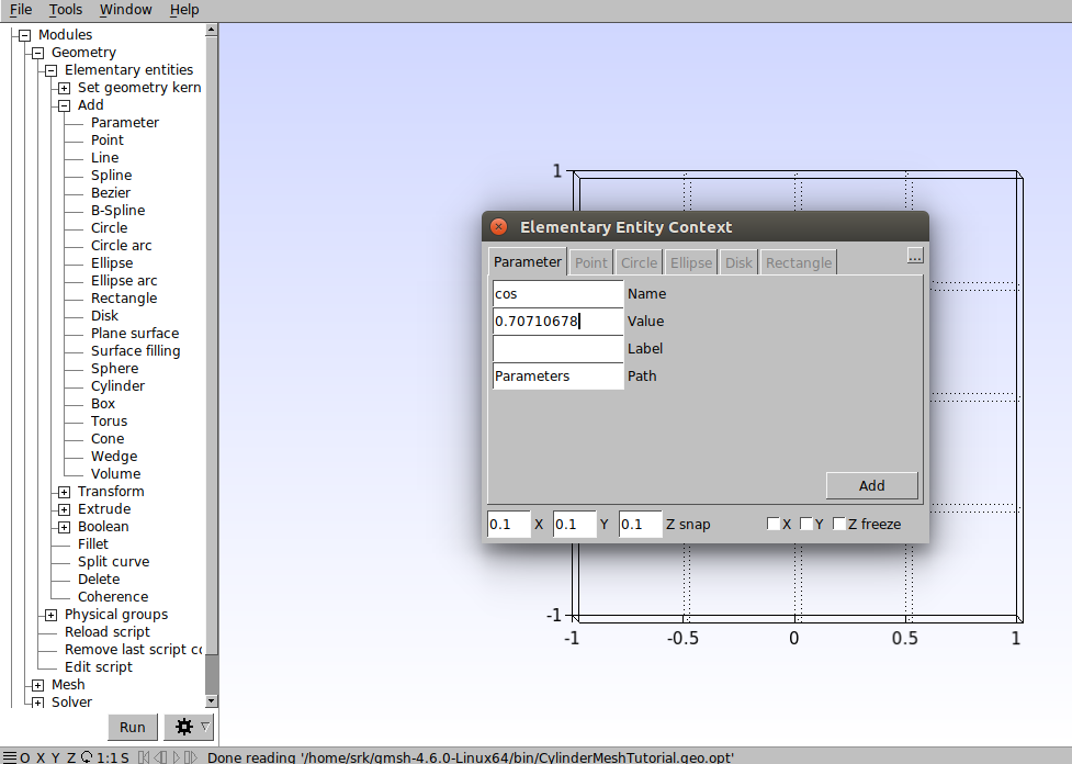
Before closing this window, add a new parameter with the name “cos” and value of 0.70710678 which is the value of cos 45° in radians. Click “Add” and close the window.
To create the parameters through the script, click on Modules→Geometry→Edit script. In the text editor, enter the following commands:
// Parameters
d = DefineNumber[ 0.05715, Name "Parameters/d" ];
//+
cos = DefineNumber[ 0.70710678, Name "Parameters/cos" ];
We will now define the points needed to build the cylinders and also the simulation domain. In the text editor, we start by inserting the center of each cylinder and then the points that dene them, as shown below. It is important to pay attention to the numbering of each point, as assigning the same number to two different points will cause errors.
// Cylinder center 1
Point(1) = {0, 0, 0, 1.0};
// Cylinder center 2
Point(2) = {3.7*d, 0, 0, 1.0};
// Points of cylinder surface 1
Point(3) = {cos*d/2, cos*d/2, 0, 1.0};
Point(4) = {-cos*d/2, cos*d/2, 0, 1.0};
Point(5) = {-cos*d/2, -cos*d/2, 0, 1.0};
Point(6) = {cos*d/2, -cos*d/2, 0, 1.0};
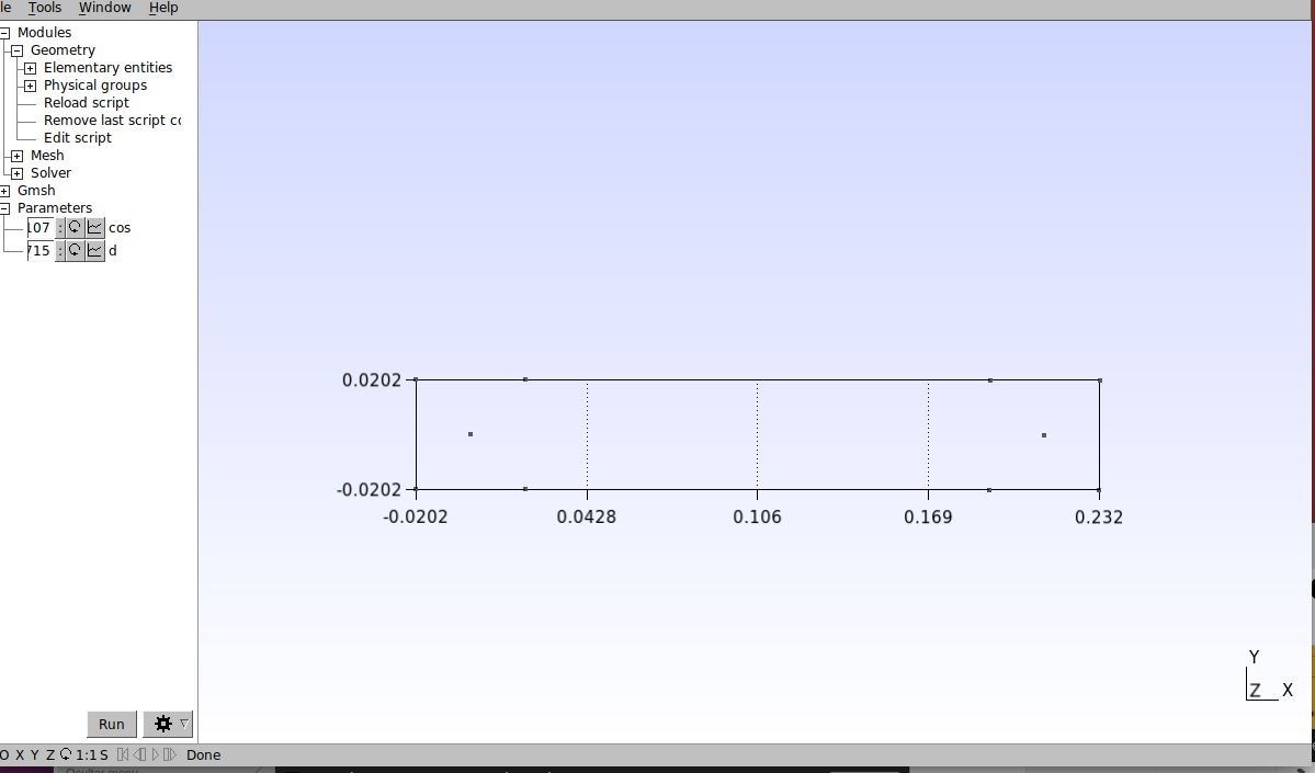
// Points of cylinder surface 2Point(7) = {cos*d/2 + 3.7*d, cos*d/2, 0, 1.0};Point(8) = {-cos*d/2 + 3.7*d, cos*d/2, 0, 1.0};Point(9) = {-cos*d/2 + 3.7*d, -cos*d/2, 0, 1.0};Point(10) = {cos*d/2 + 3.7*d, -cos*d/2, 0, 1.0};Save the script and go to Gmsh, then click on Modules→Geometry→Reload script to apply changes made in the text editor (this procedure must be repeated whenever you modify the script in the text editor). The result of these settings should be as follows:
Let’s now define the domain boundaries. Open the text editor and dena the following points:
// Domain boundary points
Point(11) = {-0.75, 0.75, 0, 1.0};
Point(12) = {-0.75, -0.75, 0, 1.0};
Point(13) = {2, 0.75, 0, 1.0};
Point(14) = {2, -0.75, 0, 1.0};
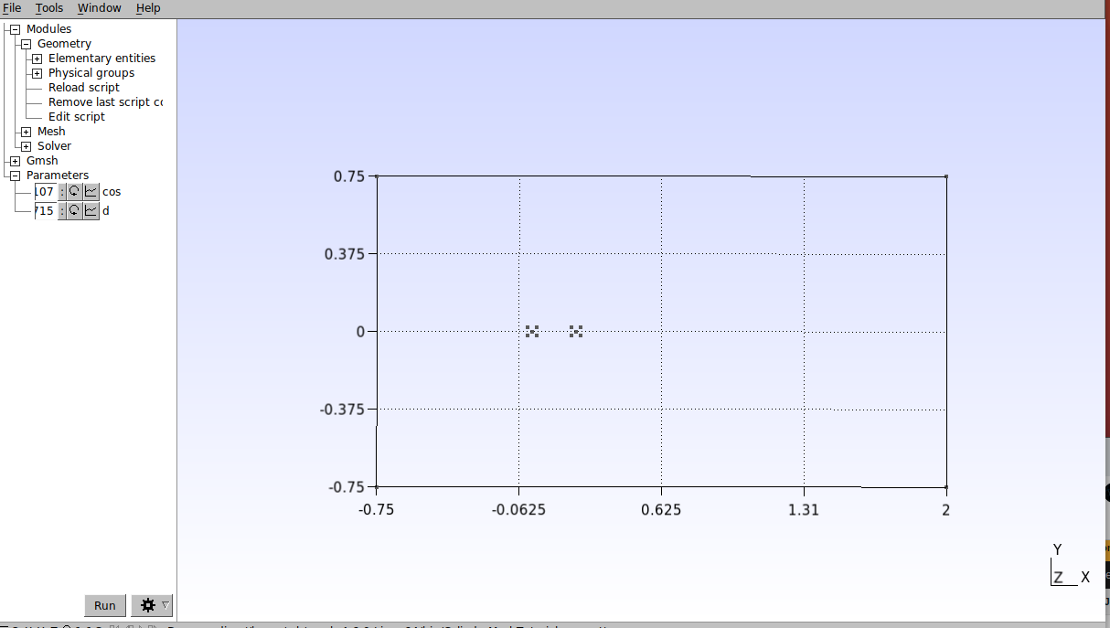
Save and reload the script. The result should be as follows.
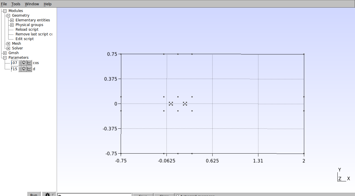
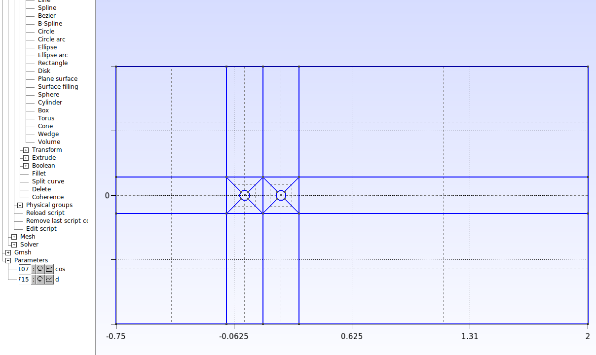
Next, we will define the set of points needed to do the domain division. This is important for the next steps where we will re-mesh. In the text editor, enter the following points:
// Domain partition points
Point(15) = {3.7*d/2, 3.7*d/2, 0, 1.0};
Point(16) = {3.7*d/2, -3.7*d/2, 0, 1.0};
Point(17) = {-3.7*d/2, 3.7*d/2, 0, 1.0};
Point(18) = {-3.7*d/2, -3.7*d/2, 0, 1.0};
Point(19) = {3.7*d/2 + 3.7*d, 3.7*d/2, 0, 1.0};
Point(20) = {3.7*d/2 + 3.7*d, -3.7*d/2, 0, 1.0};
Point(21) = {-0.75, 3.7*d/2, 0, 1.0};
Point(22) = {-0.75, -3.7*d/2, 0, 1.0};
Point(23) = {2, 3.7*d/2, 0, 1.0};
Point(24) = {2, -3.7*d/2, 0, 1.0};
Point(25) = {3.7*d/2, 0.75, 0, 1.0};
Point(26) = {3.7*d/2, -0.75, 0, 1.0};
Point(27) = {-3.7*d/2, 0.75, 0, 1.0};
Point(28) = {-3.7*d/2, -0.75, 0, 1.0};
Point(29) = {3.7*d/2 + 3.7*d, 0.75, 0, 1.0};
Point(30) = {3.7*d/2 + 3.7*d, -0.75, 0, 1.0};
The result should be like the one shown below:
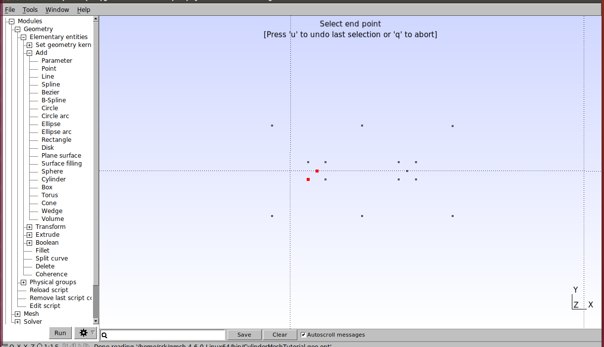
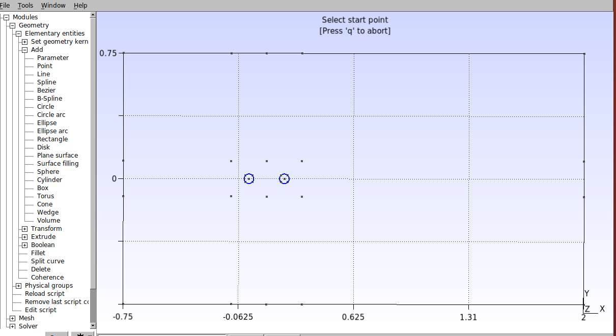
Let’s then generate the arcs that dene the cylinders. In the graphic interface, click on Modules→Geometry→Elementary entities→Add →Circle arc. Then select an outer point, then the center point and then the other outer point, as shown in the figure below.
Repeat this procedure to build the circle from the two cylinders. The result is as follows.
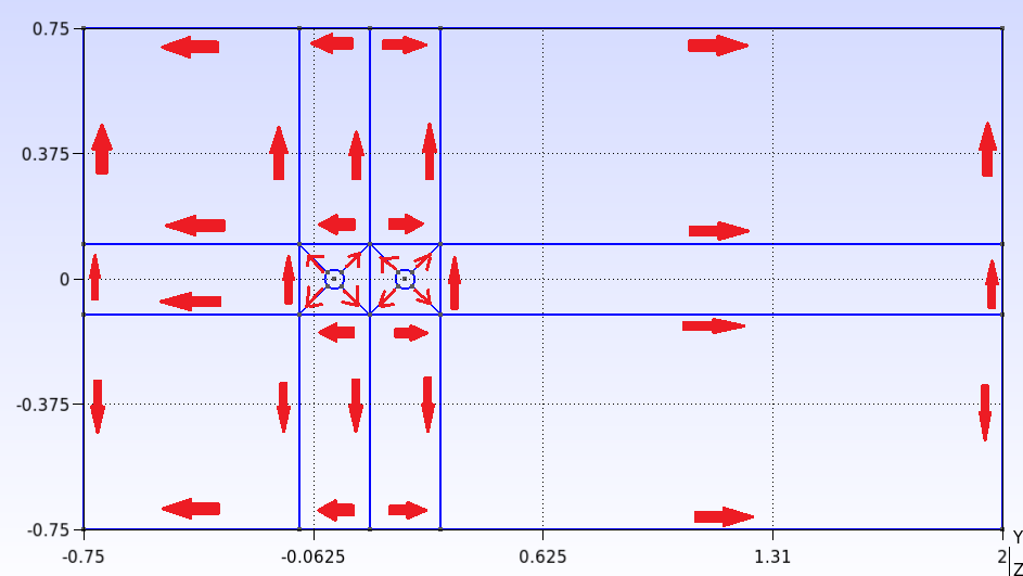
To define the lines of the domain, it is important to maintain a convention, because the order in which the points are interconnected will determine the direction of increase of the elements when we refine the mesh. First go to Modules→Geometry→Elementary entities→Add →Line. Always interconnect the points from the innermost part of the domain to the outermost part, as indicated by the arrows in the following figure
In the script, these changes are made with the following commands:
// Domain lines and arcs
Circle(1) = {5, 1, 4};
Circle(2) = {4, 1, 3};
Circle(3) = {3, 1, 6};
Circle(4) = {6, 1, 5};
Circle(5) = {9, 2, 8};
Circle(6) = {8, 2, 7};
Circle(7) = {7, 2, 10};
Circle(8) = {10, 2, 9};
Line(9) = {27, 11};
Line(10) = {17, 21};
Line(11) = {18, 22};
Line(12) = {28, 12};
Line(13) = {19, 23};
Line(14) = {29, 13};
Line(15) = {30, 14};
Line(16) = {18, 28};
Line(17) = {16, 26};
Line(18) = {20, 30};
Line(19) = {19, 29};
Line(20) = {15, 25};
Line(21) = {17, 27};
Line(22) = {20, 24};
Line(23) = {21, 11};
Line(24) = {22, 12};
Line(25) = {22, 21};
Line(26) = {18, 17};
Line(27) = {16, 15};
Line(28) = {20, 19};
Line(29) = {17, 15};
Line(30) = {18, 16};
Line(31) = {16, 20};
Line(32) = {15, 19};
Line(33) = {27, 25};
Line(34) = {25, 29};
Line(35) = {23, 13};
Line(36) = {24, 14};
Line(37) = {24, 23};
Line(38) = {28, 26};
Line(39) = {26, 30};
Line(40) = {4, 17};
Line(41) = {3, 15};
Line(42) = {5, 18};
Line(43) = {6, 16};
Line(44) = {9, 16};
Line(45) = {10, 20};
Line(46) = {7, 19};
Line(47) = {8, 15};
The next step is to define the surfaces. Click on Modules→Geometry→Elementary entities→Add →Plane Surface and select the four lines that dene each surface, as shown below. Then press the “e” key to confirm the selection and, thus, dashed lines should appear inside the surface.

Repeat this procedure for all surfaces. The result should be the following:
Now let’s recombine the surfaces to get a structured mesh. Click on Modules→Mesh→Define→Recombine. Then select all surfaces as shown below and then press the “e” key to confirm.
In the script, these procedures are done with the commands below:
// Create Surfaces
Curve Loop(1) = {21, 9, -23, -10};
Plane Surface(1) = {1};
Curve Loop(2) = {21, 33, -20, -29};
Plane Surface(2) = {2};
Curve Loop(3) = {20, 34, -19, -32};
Plane Surface(3) = {3};
Curve Loop(4) = {19, 14, -35, -13};
Plane Surface(4) = {4};
Curve Loop(5) = {13, -37, -22, 28};
Plane Surface(5) = {5};
Curve Loop(6) = {22, 36, -15, -18};
Plane Surface(6) = {6};
Curve Loop(7) = {18, -39, -17, 31};
Plane Surface(7) = {7};
Curve Loop(8) = {17, -38, -16, 30};
Plane Surface(8) = {8};
Curve Loop(9) = {16, 12, -24, -11};
Plane Surface(9) = {9};
Curve Loop(10) = {11, 25, -10, -26};
Plane Surface(10) = {10};
Curve Loop(11) = {26, -40, -1, 42};
Plane Surface(11) = {11};
Curve Loop(12) = {4, 42, 30, -43};
Plane Surface(12) = {12};
Curve Loop(13) = {43, 27, -41, 3};
Plane Surface(13) = {13};
Curve Loop(14) = {2, 41, -29, -40};
Plane Surface(14) = {14};
Curve Loop(15) = {27, -47, -5, 44};
Plane Surface(15) = {15};
Curve Loop(16) = {44, 31, -45, 8};
Plane Surface(16) = {16};
Curve Loop(17) = {45, 28, -46, 7};
Plane Surface(17) = {17};
Curve Loop(18) = {46, -32, -47, 6};
Plane Surface(18) = {18};
Recombine Surface {1, 2, 3, 4, 5, 6, 7, 8, 9, 10, 11, 14, 13, 12, 15, 18, 17, 16};
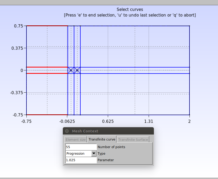
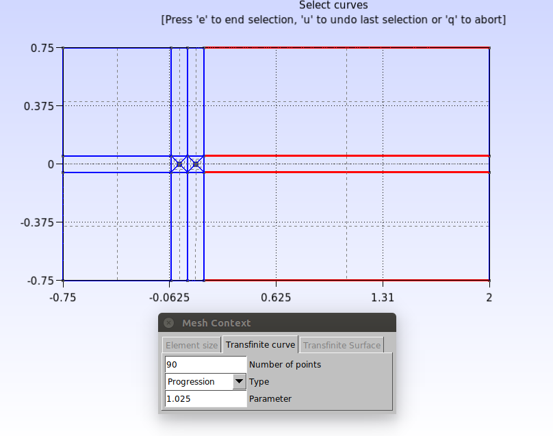
To define the increase rates of the elements, we will use the “Transnite” function. Click on Modules→Mesh→Define→Transfinite→Curve. Enter the number of points and the increase parameter that appear in the “Mesh context” window and then select the lines as shown in the figure below. After that, press the “e” key to confirm.
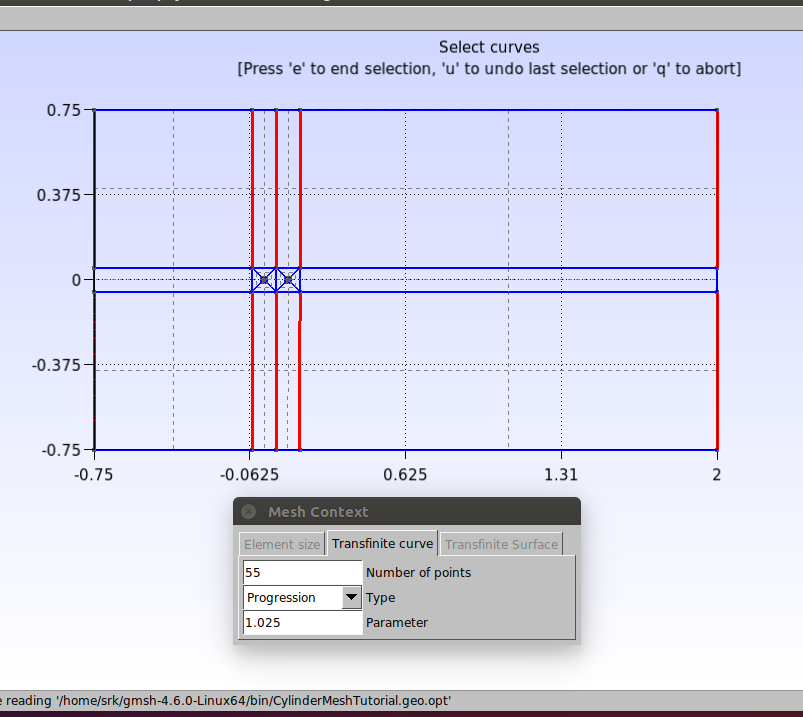
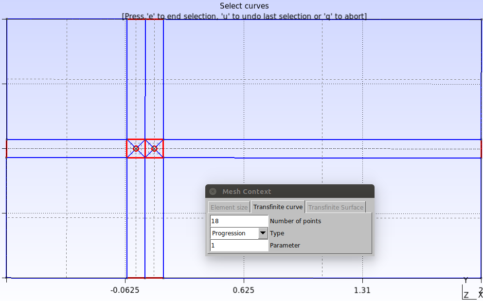
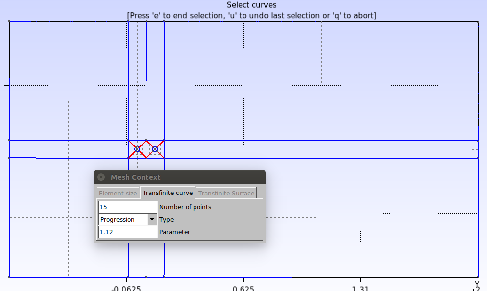
Repeat this procedure for all remaining curves as indicated by the figures below.
In the script this is done as follows:
Transfinite Curve {23, 21, 20, 19, 35, 24, 16, 17, 18, 36} = 55 Using Progression 1.025;
Transfinite Curve {9, 10, 11, 12} = 55 Using Progression 1.025;
Transfinite Curve {14, 13, 22, 15} = 90 Using Progression 1.025;
Transfinite Curve {1, 26, 25, 2, 29, 33, 4, 30, 38, 8, 31, 39, 6, 32, 34, 7, 28, 37, 3, 27, 5} = 18 Using Progression 1;
Transfinite Curve {40, 42, 43, 41, 47, 44, 45, 46} = 15 Using Progression 1.12;
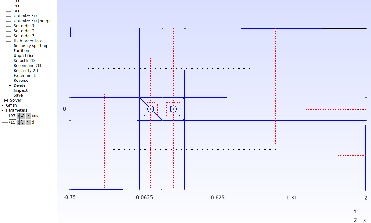
Now let’s apply the “Transnite” function to each surface. Click on Modules→Mesh→Define→Transfinite→Surface and select the surface by clicking on the dashed lines inside it, as shown in the figure below, and press “e” to confirm.
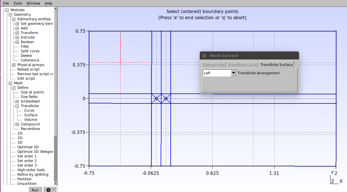
Repeat this procedure for all surfaces. The script must have the following commands:
Transfinite Surface {1};
Transfinite Surface {2};
Transfinite Surface {3};
Transfinite Surface {4};
Transfinite Surface {5};
Transfinite Surface {6};
Transfinite Surface {7};
Transfinite Surface {8};
Transfinite Surface {9};
Transfinite Surface {10};
Transfinite Surface {11};
Transfinite Surface {14};
Transfinite Surface {13};
Transfinite Surface {12};
Transfinite Surface {15};
Transfinite Surface {18};
Transfinite Surface {17};
Transfinite Surface {16};
The next step is to extrude the mesh. Click on Modules→Geometry→Elementary entities→Add→Extrude→Translate. In the window, set the values as indicated in the figure below and check the “Extrude mesh” option. Then select all surfaces and press “e” to confirm.
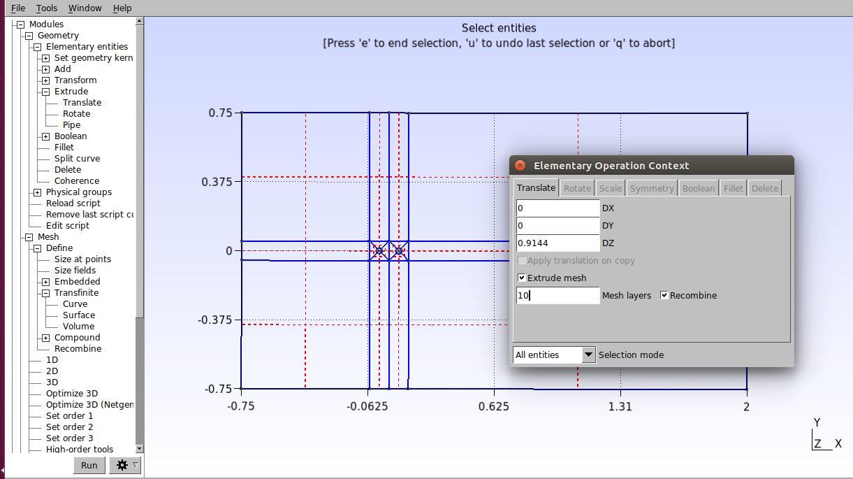
In the script, enter the following commands:
Extrude {0, 0, 0.9144} {
Surface{1}; Surface{2}; Surface{3}; Surface{4}; Surface{10}; Surface{11}; Surface{14}; Surface{12}; Surface{13}; Surface{15}; Surface{18}; Surface{17}; Surface{16}; Surface{5}; Surface{6}; Surface{7}; Surface{8}; Surface{9}; Layers{10}; Recombine;
}
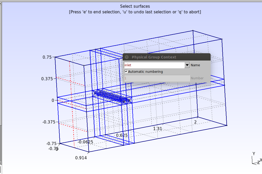
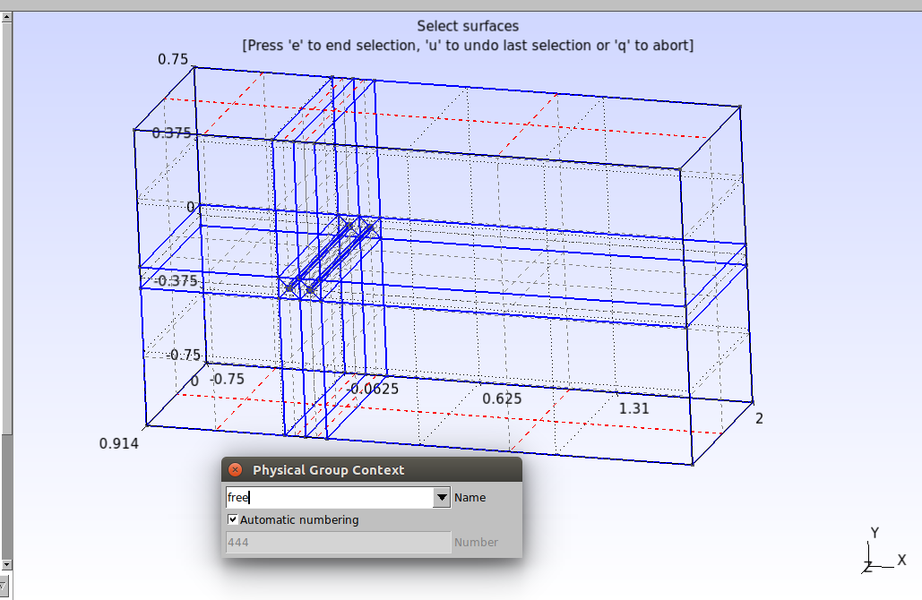
Finally, let’s define the faces that will be responsible for the boundary conditions in the simulation. Click on Modules→Geometry→Physical groups→Add→Surface. In the window that opens, type the name “inlet”, select the three input surfaces as shown in the image below and then press the “e” key to confirm.
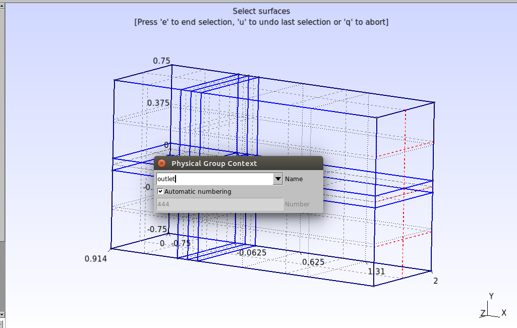
Repeat the procedure for the other groups, as shown in the images below
Output:
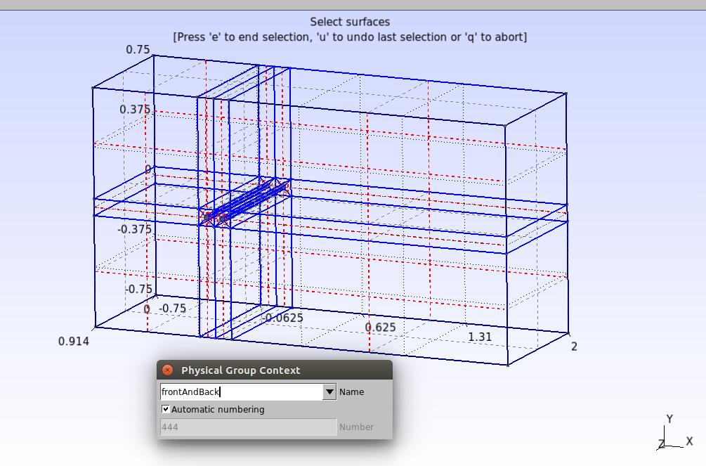
Front and back sides:
Bottom and top sides:
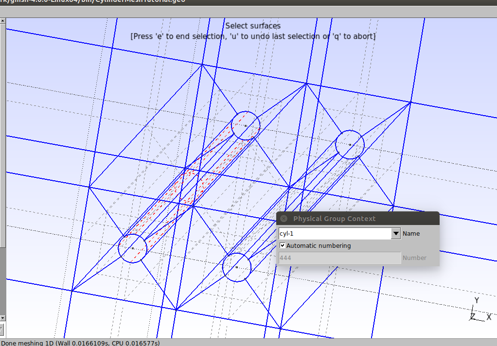
The four surfaces of cylinder 1:
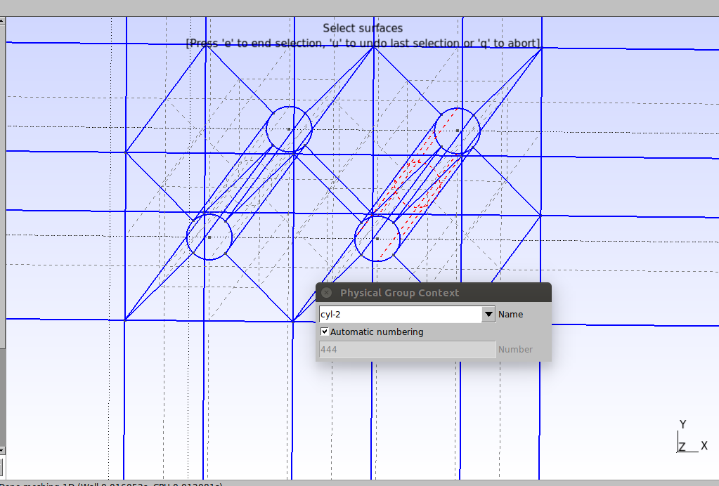
The four surfaces of cylinder 2:
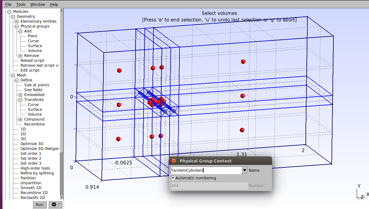
Now click on Modules→Geometry→Physical groups→Add→Volume and in the window that opens type “TandemCylinders” as the name and then select all the spheres as shown below. Press the “e” key to confirm.
In the script, this is done by the following commands:
Physical Surface("inlet") = {64, 148, 438};
Physical Surface("outlet") = {130, 346, 368};
Physical Surface("frontAndBack") = {69, 91, 113, 135, 355, 377, 399, 421, 443, 157, 179, 201, 245, 223, 267, 289, 311, 333, 4, 5, 6, 7, 8, 9, 10, 1, 2, 3, 15, 18, 17, 16, 13, 14, 11, 12};
Physical Surface("free") = {126, 104, 82, 60, 372, 390, 412, 434};
Physical Surface("cyl-1") = {210, 174, 188, 244};
Physical Surface("cyl-2") = {262, 332, 310, 288};
Physical Volume("TandemCylinders") = {1, 2, 3, 4, 5, 6, 7, 9, 8, 10, 11, 12, 13, 14, 15, 16, 17, 18};
The mesh configurations are now ready. To generate it click on Modules→Mesh→3D. The result should be the following:

Note: if the mesh elements are not shown when doing the above procedure, double click on the coordinate axis at the bottom right, as shown above, and click on “Mesh visibility” and check the option “2D element edges”.
To export the mesh go to the top bar in Gmsh in File→Export and save it with the name “TandemCylinders.msh”. In the window that opens, choose the “Version 2 ASCII” format as shown below and click “Ok”.
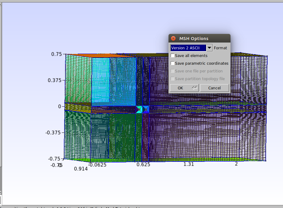
Now, the “TandemCylinders.msh” file can now be imported into OpenFOAM.
Generation of the surfaces used in the acoustic analogy
To perform the simulation of the case (tutorial), along with acoustic analogies, it is necessary to generate surfaces that encompass the noise sources. Let’s generate these surfaces in Gmsh.
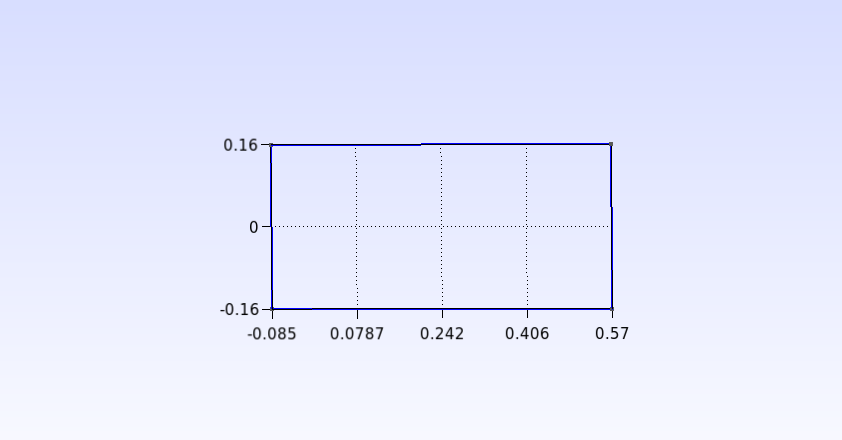
First, create a new file by clicking File→New. Let’s create the surface points. Click on Modules→Geometry→Edit script and enter the following points:
Point(1) = {-0.085, 0.16, 0, 1.0};
Point(2) = {-0.085, -0.16, 0, 1.0};
Point(3) = {0.57, 0.16, 0, 1.0};
Point(4) = {0.57, -0.16, 0, 1.0};
Save the script and then in Gmsh click on Modules→Geometry→Reload script.
Let’s join the dots to form a rectangle. Click on Modules→Geometry→Elementary entities→Add→Line. Click on two points to generate a line (As we are not going to use increase rate in this case, the points can be connected in any order). In the end you should get the following result:
To create the surface click on Modules→Geometry→Elementary entities→Add→Plane Surface. Select all the lines that form the rectangle, as shown below, and press “e” to confirm.
Now apply the “Recombine” function by clicking on Modules→Mesh→Define→Recombine. Select the surface by clicking on the dashed lines and press “e” to confirm.

Let’s apply the “Transnite” function to reno the mesh. click on Modules→Mesh→Define→Transfinite→Curve. In the window that opens, set the number of points to 70, select the horizontal lines and press “e” to confirm.
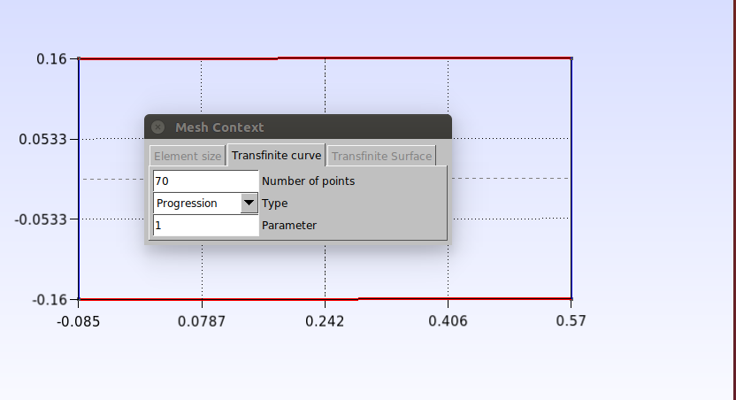
Then, with the window still open, change the number of points to 40, select the vertical lines and press “e” to confirm.

Now click on Modules→Mesh→Define→Transfinite→Surface, sselect the surface by clicking on the dashed lines and press “e” to confirm.
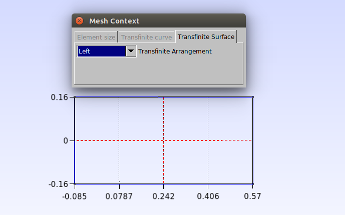
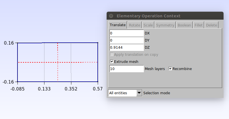
The next step is to extrude the surface. Click on Modules→Geometry→Elementary entities→Extrude→ Translate. In the window that opens, set the values as shown below, select the surface by clicking on the dashed lines inside the surface and press “e” to confirm.
The final surface script looks like this:
Point(1) = {-0.085, 0.16, 0, 1.0};
Point(2) = {-0.085, -0.16, 0, 1.0};
Point(3) = {0.57, 0.16, 0, 1.0};
Point(4) = {0.57, -0.16, 0, 1.0};
Line(1) = {1, 3};
Line(2) = {3, 4};
Line(3) = {4, 2};
Line(4) = {2, 1};
Curve Loop(1) = {1, 2, 3, 4};
Plane Surface(1) = {1};
Recombine Surface {1};
Transfinite Curve {1, 3} = 70 Using Progression 1;
Transfinite Curve {4, 2} = 40 Using Progression 1;
Transfinite Surface {1};
Extrude {0, 0, 0.9144} {
Surface{1}; Layers{10}; Recombine;
}
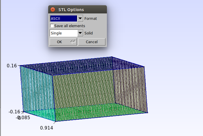
To create the three-dimensional mesh surface click on Modules→Mesh→3D. To export it, go to File→Export. Put the file name as “surface1.stl”, choose the location where it will be saved and click “Save”. In the “STL Options” window that opens, make sure to select the options as shown below.
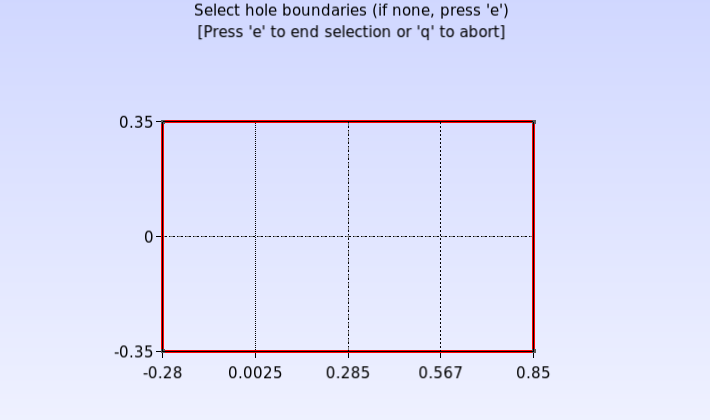
The second surface to be used is similar to the first. From the first script, change the position of the points and also the number of points used in the “Transnite” function as shown below
Point(1) = {-0.28, 0.35, 0, 1.0};
Point(2) = {-0.28, -0.35, 0, 1.0};
Point(3) = {0.85, 0.35, 0, 1.0};
Point(4) = {0.85, -0.35, 0, 1.0};
Line(1) = {1, 3};
Line(2) = {3, 4};
Line(3) = {4, 2};
Line(4) = {2, 1};
Curve Loop(1) = {1, 2, 3, 4};
Plane Surface(1) = {1};
Recombine Surface {1};
Transfinite Curve {1, 3} = 90 Using Progression 1;
Transfinite Curve {4, 2} = 55 Using Progression 1;
Transfinite Surface {1};
Extrude {0, 0, 0.9144} {
Surface{1}; Layers{10}; Recombine;
}
Reload the script and to finish, repeat the process of creating the 3D mesh and exporting it as described for surface 1. Save it with the name “surface2.stl”.


