Simulation of a 3D Dipole in OpenFoam Using LibAcoustics Library


Simulation of a 3D dipole in OpenFOAM using the libAcoustics library
Note:
- This tutorial has only didactic purpose, aiming to help beginners, and it does not guarantee quality of simulation results. Verification and validation of the results, and also the study of mesh refinement and other analyzes are left as responsibility of the user.
- This offering is not approved or endorsed by OpenCFD Limited, producer and distributor of the OpenFOAM software via www.openfoam.com, and owner of the OPENFOAM® and OpenCFD® trade marks.
- This tutorial was created within the context of an UFSC extension project and it is not approved by GMSH, LibAcoustics and OpenFOAM® developers.
- OpenFOAM version 1912 was used.
- This tutorial was prepared by the undegraduate students Julio Victor Viera, under the supervision of Filipe Dutra da Silva.
- Please quote this page if you use this material. Questions and suggestions can be sent to the contact addresses shown at the end of this page.
This tutorial aims to show some functionalities of the acoustic library libAcoustics created by Epikhin et al. for OpenFOAM, using a 3D dipole case. This library contains the implementation of acoustic analogies that allow the calculation of noise in far-field from data collected close to the source. Here we will make use of the Williams-Hawkings analogy.
First, the acoustic pressure in the time domain is calculated. Then, these data are converted to the frequency domain using the Fast Fourier Transform (FFT) algorithm.
Note: Before installing the libAcoustics library, you must have installed the FFTW library.
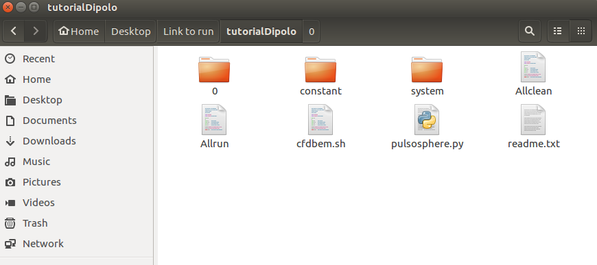
To start, copy the “monopole3D” case present in the “Tutorials” folder that comes with the installation files of the library and paste it in the desired directory with the name “tutorialDipolo”. The folder must contain the following files:
Open the “system” folder and then the “controlDict” file. Let’s use the “rhoPimpleFoam” solver. Change the value of “deltaT” to 2.5e-4, the value of “endTime” to 0.13, and the value of “maxDeltaT” to 1e-3, as shown below. The inserted functions belong to the libAcoustics library.
application rhoPimpleFoam;
startFrom startTime;
startTime 0;
stopAt endTime;
endTime 0.13;
deltaT 2.5e-4;
writeControl adjustableRunTime;
writeInterval 5e-3;
purgeWrite 200;
writeFormat ascii;
writePrecision 9;
writeCompression on;
timeFormat general;
timePrecision 6;
runTimeModifiable true;
adjustTimeStep false;
maxCo 0.5;
maxDeltaT 1e-3;
functions
{
    #include "probeControl"
    #include "fwhControl"
    #include "sphereAverage"
    #include "soundPressureSampling"
}
After applying the necessary changes, save them and close the file. Next, open the “fwhCommonSettings” file. In it are contained the configurations of the acoustic analogy used, known as Ffowcs Williams-Hawkings (FWH). Change the “timeStart” to 0.001. Change the propagation velocity (c0) and density (rhoInf) to the values for air, as indicated below. The “dRef” is used in 2D simulations to define the thickness of the domain, but as our case is 3D, change the value to -1 to ignore this function. The positions in the far field where you want to make noise measurements must be configured in “observers”.
libs (“libAcoustics.so”);
log             true;
writeFft        true;
probeFrequency  1;
timeStart       0.001;
timeEnd         0.13;
c0              340;
dRef            -1;
pName           p;
pInf            101325;
rho             rho;
rhoInf          1.22;
CofR            (0 0 0);

observers
{
    R-A
    {
        position    (0 0 1.0);
        pRef        2.0e-5;
        fftFreq     512;
    }
    R-B
    {
        position    (0 0 2.0);
        pRef        2.0e-5;
        fftFreq     512;
    }
    R-C
    {
        position    (0 0 3.0);
        pRef        2.0e-5;
        fftFreq     512;
    }
    R-D
    {
        position    (0 0 4.0);
        pRef        2.0e-5;
        fftFreq     512;
    }
    R-E
    {
        position    (0 0 5.0);
        pRef        2.0e-5;
        fftFreq     512;
    }
    R-F
    {
        position    (0 0 10.0);
        pRef        2.0e-5;
        fftFreq     512;
    }
}
In the “fwhControl” file are the configurations of the surfaces that collect the data in the regions close to the source. We will use the same surfaces as in the monopole case. These surfaces enclose the entire sphere. They are located in the constant/triSurface folder and must be in the format .stl.
In the “decomposeParDict” file, change the value of “numberOfSubdomains” to the number of processors you want to use in the parallel simulation.
The other files in the “system” folder will not be changed. Now leave the “system” folder and enter the “constant” folder. Open the “thermophysicalProperties” file and modify the values as shown below. After that, save the file and close it. Still inside the “constant” folder, change the name of the folder “polyMesh0” to “polyMesh” (just remove the “0”).
thermoType
{
type hePsiThermo;
mixture pureMixture;
transport const;
thermo hConst;
equationOfState perfectGas;
specie specie;
energy sensibleEnthalpy;
}
mixture
{
specie
{
nMoles 1;
molWeight 28.9;
}
thermodynamics
{
Cp 1005;
Hf 0;
}
transport
{
mu 1.8e-05;
Pr 0.7;
}
}
The next step is to configure the boundary conditions. Leave the “constant” folder and open the “0” folder and then open the “U” file. This is where we are going to change the configuration of a monopole to the configuration of a dipole. We can define a dipole as a monopole that oscillates in only one direction. To do this, change the “sphere” settings to the ones below.
dimensions [0 1 -1 0 0 0 0];
internalField uniform (0 0 0);
boundaryField
{
free
{
type waveTransmissive;
field U;
phi phi;
rho rho;
psi thermo:psi;
gamma 1.4;
value uniform (0 0 0);
}
sphere
{
    type            uniformFixedValue;
    uniformValue    sine;
    uniformValueCoeffs
    {
        amplitude   0.01;
        scale       (0 0 1);
        level       (0 0 0);
        frequency   constant 100;
    }
}

#include "cyc"
}
Note: The boundary condition “waveTransmissive” present in “free” is used to avoid the reflection of waves at the boundaries of the computational domain.
The other boundary conditions are kept the same as in the monopole case.
With the case settings ready, open the terminal and go to the “tutorialDipolo” folder, type “decomposePar” and press enter to divide the domain, since we are going to run the simulation in parallel.

So, we can start running the simulation. For that type “mpirun -np 5 rhoPimpleFoam -parallel > log &” and press enter (replace the number 5 with the number of processors you configured in the “decomposeParDict” file).

Post processing
After finishing the simulation, go to the terminal and type “reconstructPar -latestTime” to reconstruct the last time-step of the simulation.
.

Next, let’s create a file that can be read in Paraview. To do this, type “nano dipolo.foam”, then press “enter”, then ctrl+o, “enter” and finally ctrl+x.

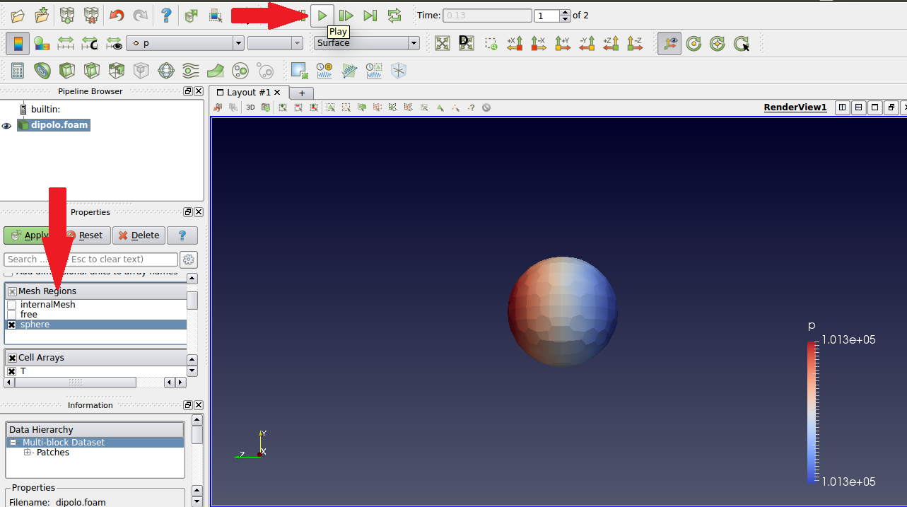
Type “paraview dipolo.foam” to view the result in Paraview.

Click on advance to the last time-step and then uncheck the “internalMesh” option in the left bar and check the “sphere” option, as indicated in the image below. Click “Apply” to view the result.
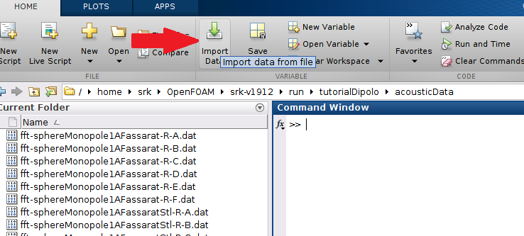
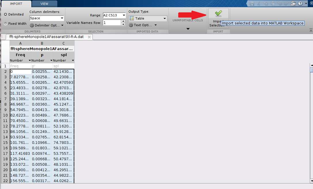
The acoustic simulation data is saved in the “acousticData” folder inside the “tutorialDipolo” folder. Here, will be presented a code in Matlab that plots the results of acoustic pressure as a function of time and also the frequency spectrum for microphone A.
First, click on the “Import Data” option as shown below and select the file “fft-sphereMonopole1AFassaratStl-R-A.dat”. In the window that opens, click on “Import Selection”. Do the same procedure to import the “sphereMonopole1AFassarat-time.dat” file.
To plot the graphs, just run the following script:
t = sphereMonopole1AFassaratStltime{:,1};
p = sphereMonopole1AFassaratStltime{:,2};
f = fftsphereMonopole1AFassaratStlRA{1:256,1};
spl = fftsphereMonopole1AFassaratStlRA{1:256,3};
figure(1)
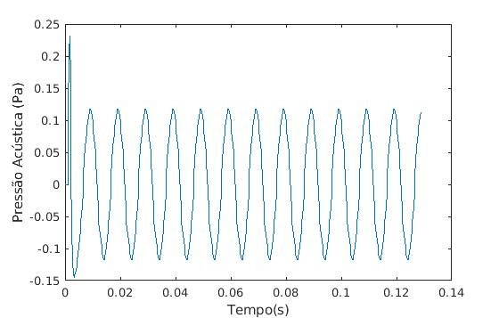
plot(t,p)
xlabel(“Tempo(s)”)
ylabel(“Pressão Acústica (Pa)”)
figure(2)
semilogx(f,spl)
xlabel(“Frequência (Hz)”)
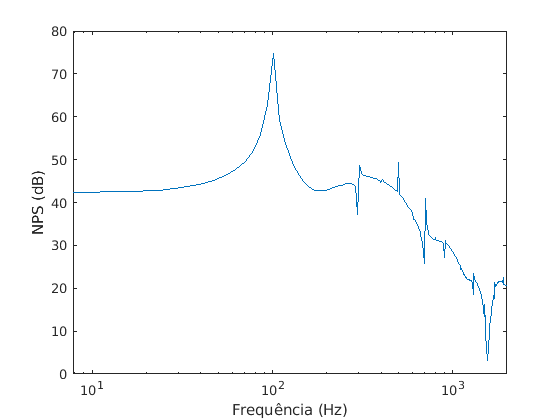
ylabel(“NPS (dB)”)
Sound pressure as a function of time:
Frequency spectrum: