

Mesh Generation Tutorial of Axisymmetric Nozzle


Mesh Generation Tutorial of Axisymmetric Nozzle
Note:
- This tutorial has only didactic purpose, aiming to help beginners, and it does not guarantee quality of simulation results. Verification and validation of the results, and also the study of mesh refinement and other analyzes are left as responsibility of the user.
- This offering is not approved or endorsed by OpenCFD Limited, producer and distributor of the OpenFOAM software via www.openfoam.com, and owner of the OPENFOAM® and OpenCFD® trade marks.
- This tutorial was created within the context of an UFSC extension project and it is not approved by GMSH and OpenFOAM® developers.
- This tutorial was prepared by the undergraduate student Juliano Simon and Widmark Kauê Silva Cardoso under the supervision of Filipe Dutra da Silva.
- Please quote this page if you use this material. Questions and suggestions can be sent to the contact addresses shown at the end of this page.
In this tutorial it will be presented the process of creating a mesh and a structured mesh for the simulation of flow in an axisymmetric nozzle using the Gmsh code.
There are two ways of using Gmsh: through the commands of the graphical interface of the software or editing the script with extension .geo, which is generated by the software. Both ways of using the software will be shown here. To open the script, go to Modules→Geometry and click on Edit script.
The first step is the declaration of geometry coordinates. In the file .geo type the geometry coordinates in the format “Point(1) = (0,0,0,1.0);”, where the first three terms are, respectively, x, y and z coordinates. Thus, the file should have the following setting:
// SETTING THE POINTS:
Point(1) = {-0.254,0,0,1.0};
Point(2) = {-0.199,0,0,1.0};
Point(3) = {0,0,0,1.0};
Point(4) = {2.496,0,0,1.0};

// Nozzle points:
Point(5) = {-0.254,0.076,0,1.0};
Point(6) = {-0.199,0.076,0,1.0};
Point(7) = {-0.185,0.071,0,1.0};
Point(8) = {-0.139,0.047,0,1.0};
Point(9) = {-0.083,0.032,0,1.0};
Point(10) = {0,0.025,0,1.0};
Point(11) = {-0.254,0.077,0,1.0};
Point(12) = {-0.199,0.077,0,1.0};
Point(13) = {-0.185,0.072,0,1.0};
Point(14) = {-0.139,0.048,0,1.0};
Point(15) = {-0.083,0.033,0,1.0};

//-----
Point(16) = {2.496,0.3762,0,1.0};
Point(17) = {-0.254,0.6,0,1.0};
Point(18) = {-0.199,0.608,0,1.0};
Point(19) = {0,0.6369,0,1.0};
Point(20) = {2.496,1,0,1.0};
//================================
Save the file. In the graphical interface, click on Modules→Geometry → Reload script (repeat this process whenever you make any modification in the .geo file). The result is shown in the figure below.
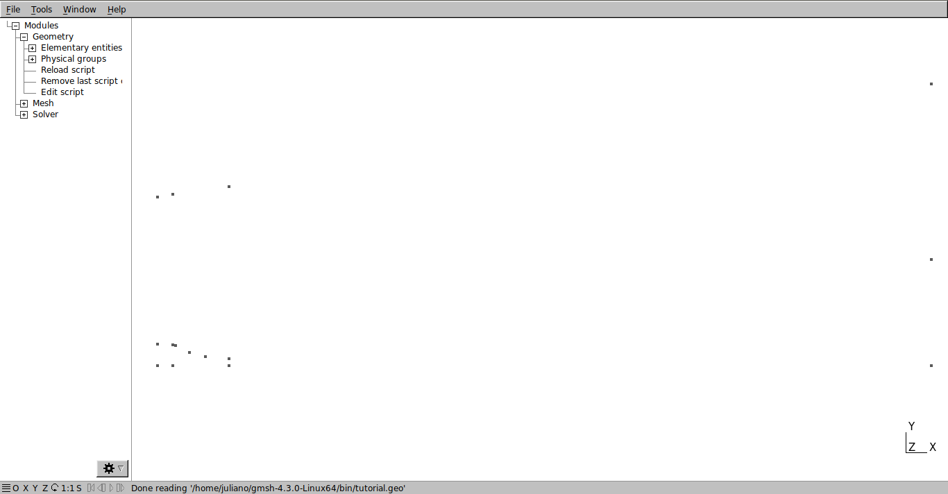
Note: To create the points using graphical interface, go to Modules→Geometry → Elementary entities → Add → Point.
Observe in this example that the points which define the inner and outer surfaces of the nozzle are very close. This is done to create a small thickness in the nozzle.
It is very important to keep consistency in the numbering of the points. There can’t be two points with the same number, and the numbering of the points is used to create the other parts of the geometry. Thus, the organization of the code is crucial to facilitate the work. If necessary, the numbering of the points can be shown in the graphical interface by the command Tools → Options → Geometry and clicking on Point labels.
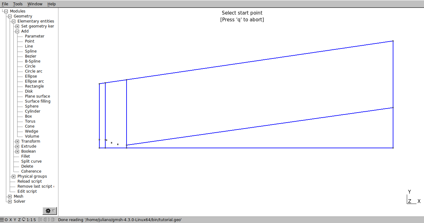
The straight lines that define the domain of simulation and the blocks of the mesh can be generated by script, adding the command “Line(1) = {1,2};”, where 1 and 2 are the points that will be connected. Repeat this process until you connect all the desired points. The result in the .geo file and in the graphical interface should be like shown below.
Note: to join the points in the graphical interface, use the too Modules→Geometry → Elementary entities → Add → Line and select the points that have to be connected.
// SETTING THE LINES:

//+
Line(1) = {1, 2};
//+
Line(2) = {2, 3};
//+
Line(3) = {3, 4};
//+
Line(4) = {4, 16};
//+
Line(5) = {16, 20};

//+
Line(6) = {20, 19};
//+
Line(7) = {19, 18};
//+
Line(8) = {18, 17};
//+
Line(9) = {17, 11};
//+
Line(10) = {5, 1};
//+
Line(11) = {2, 6};
//+
Line(12) = {12, 18};
//+
Line(13) = {3, 10};
//+
Line(14) = {10, 19};
//+
Line(15) = {10, 16};
The nozzle contour will be defined in two parts. The first with a straight line and the second with a spline. Sometimes the characteristics of the spline require the setting of a large number of points in order to get the shape of the nozzle. First we connect the two points of the flat part of the nozzle with a line.
To create a spline in the script, type “Spline(nº) = {6, 7, 8, 9, 10};” (the spline has the same numbering as the lines). The numbers in curly braces represent the points that will be connected according to the order in which they are typed.
Note: To define the spline in the graphical interface, go to Modules→Geometry → Elementary entities → Add → Spline and select all the points you want to connect and press the “e” key to confirm.
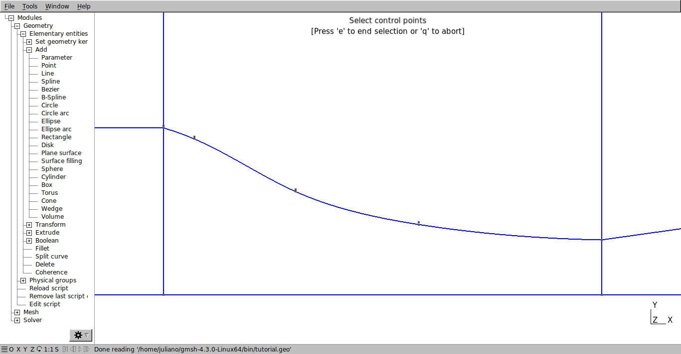
Repeat the same process with the outside of the nozzle.
// Setting the lines of the nozzle:
//+
Line(16) = {5, 6};
//+
Spline(17) = {6, 7, 8, 9, 10};

//+
Line(18) = {11, 12};
//+
Spline(19) = {12, 13, 14, 15, 10};
//================================
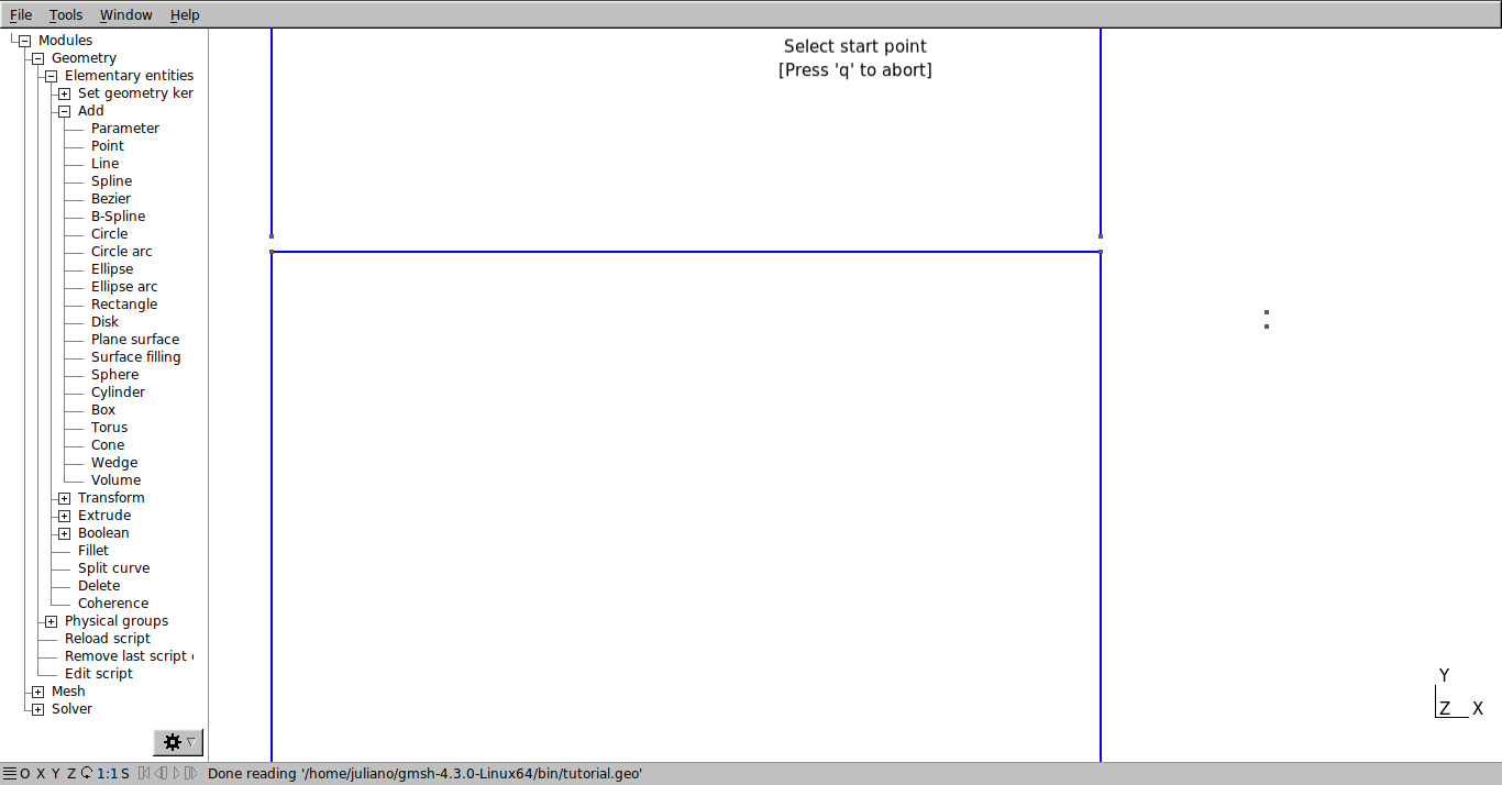
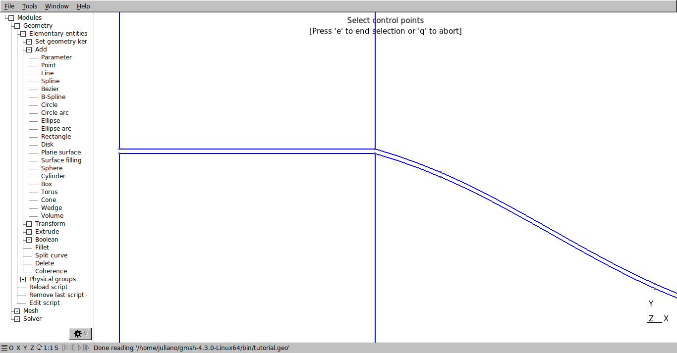
Now we are going to define the surfaces. Select Modules→Geometry → Elementary entities → Add → Plane surface. To define a surface, four lines must be selected. It is important to note that surfaces with three or more lines also can be created. However, to generate a structured mesh, the surfaces of mesh blocks must be defined in this manner. This explains the divisions made in the domain earlier.
Select the four lines that will define each surface and press the “e” key to confirm. If the process was done correctly, dotted lines should appear inside the surfaces.
In the .geo script, the definition of surfaces should be as shown below.
//SETTING THE SURFACES:
//+
Curve Loop(1) = {1, 11, -16, 10};
//+
Plane Surface(1) = {1};
//+
Curve Loop(2) = {11, 17, -13, -2};
//+
Plane Surface(2) = {2};
//+
Curve Loop(3) = {13, 15, -4, -3};
//+
Plane Surface(3) = {3};
//+
Curve Loop(4) = {9, 18, 12, 8};
//+
Plane Surface(4) = {4};
//+
Curve Loop(5) = {12, -7, -14, -19};
//+
Plane Surface(5) = {5};
//+
Curve Loop(6) = {15, 5, 6, -14};
//+
Plane Surface(6) = {6};
//+
//================================
The “Curve Loop” tool defines the lines that edge the surfaces and the “Plane Surface” creates the surface. The negative signs in the number of some lines indicate their orientations, depending on the order of the points that define them.
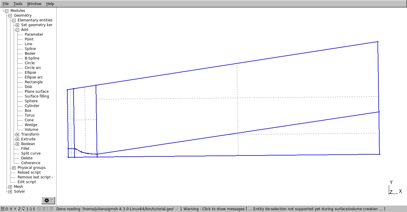
For axisymmetric simulation in OpenFOAM, it is necessary to generate a wedge domain. Moreover, it is necessary to define a symmetric domain in respect to the xy plane. Therefore, it is needed to rotate the base mesh before generating the wedge by extrusion.
Click on Modules→Geometry → Transform → Rotate and set the options like shown in the figure below.
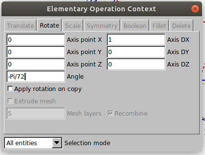
Select all the faces and press the “e” key to confirm. In this way, the geometry will be rotated by -2.5° to compensate for the extrusion of 5° that will be made later.
In the script, these changes should be as shown below.
// ROTATION:
Rotate {{1, 0, 0}, {0, 0, 0}, -Pi/72} {
Surface{1}; Surface{2}; Surface{3}; Surface{4}; Surface{5}; Surface{6};
}

//================================
For the creation of a structured mesh, Gmsh offers the “Transfinite” option that must be applied to all lines. This option allows us to define the number of volumes that your mesh will have and the increase rate of those volumes along the lines.
Click on Modules → Mesh → Define → Transfinite → Curve. The Transfinite option must be defined for each line, so it is required to keep consistency in its creation (you can make the name of the lines explicit with the same path that was used for the points) and it is recommended to use comments in the .geo file so that there is no confusion with the names. Note that, due to rotation, the name of the lines will be different from what was defined earlier. Select a line and press the “e” key to confirm. In the .geo file, the settings should be like that:
// TRANSFINITE:
//+
Transfinite Curve {20} = 10 Using Progression 1;
The value 10 indicates the number of divisions made in the mesh for that line and the value 1 indicates the size ratio between two consecutive volumes. To facilitate later editing of these values, we can replace them by variables.
// TRANSFINITE:
a=10;
//+
Transfinite Curve {20} = a Using Progression 1;
NOTE: opposite lines in the same block must have the same number of divisions for the final mesh to be structured, so it is recommended to place the same variable for these lines.
For better organization, the creation of Transfinites will follow this order: first the internal horizontal lines of the nozzle, then the external horizontal lines in front of the nozzle, the internal vertical lines, the horizontal lines of the external part of the nozzle and the vertical lines of the external part of the nozzle. Following this order, the result is like that:
// TRANSFINITE:

// internal horizontal lines of the nozzle:

a = 14;
b = 160;
//+
Transfinite Curve {20} = a Using Progression 1;
//+
Transfinite Curve {22} = a Using Progression 1;
//+
Transfinite Curve {26} = b Using Progression 1;
//+
Transfinite Curve {24} = b Using Progression 1;

// horizontal lines in front of the nozzle:

c = 225;
//+
Transfinite Curve {29} = c Using Progression 1;
//+
Transfinite Curve {27} = c Using Progression 1;
//+
Transfinite Curve {38} = c Using Progression 1;

// internal vertical lines of the nozzle:

d = 40;
//+
Transfinite Curve {23} = d Using Progression 1;
//+
Transfinite Curve {21} = d Using Progression 1;
//+
Transfinite Curve {25} = d Using Progression 1;
//+
Transfinite Curve {28} = d Using Progression 1;

// external horizontal lines of the nozzle:

e = 14;
f = 160;
//+
Transfinite Curve {31} = e Using Progression 1;
//+
Transfinite Curve {33} = e Using Progression 1;
//+
Transfinite Curve {36} = f Using Progression 1;
//+
Transfinite Curve {34} = f Using Progression 1;

// external vertical lines of the nozzle:

g = 100;
//+
Transfinite Curve {30} = g Using Progression 1;
//+
Transfinite Curve {32} = g Using Progression 1;
//+
Transfinite Curve {35} = g Using Progression 1;
//+
Transfinite Curve {37} = g Using Progression 1;
Then, it is needed to apply a Transfinite to the surfaces. Click on Modules → Mesh → Define → Transfinite → Surface. Select each surface and press “e” to confirm. Then, go to Modules → Mesh → Define → Recombine and select all the surfaces and press “e” to confirm. The result in the .geo file is shown below.
//+
Transfinite Surface {1};
//+
Transfinite Surface {2};
//+
Transfinite Surface {3};
//+
Transfinite Surface {4};
//+
Transfinite Surface {5};
//+
Transfinite Surface {6};
//+
Recombine Surface {1, 2, 3, 4, 5, 6};
//=================================
Now the 2D mesh can be viewed by clicking on Modules → Mesh → 2D. The result should be like that:
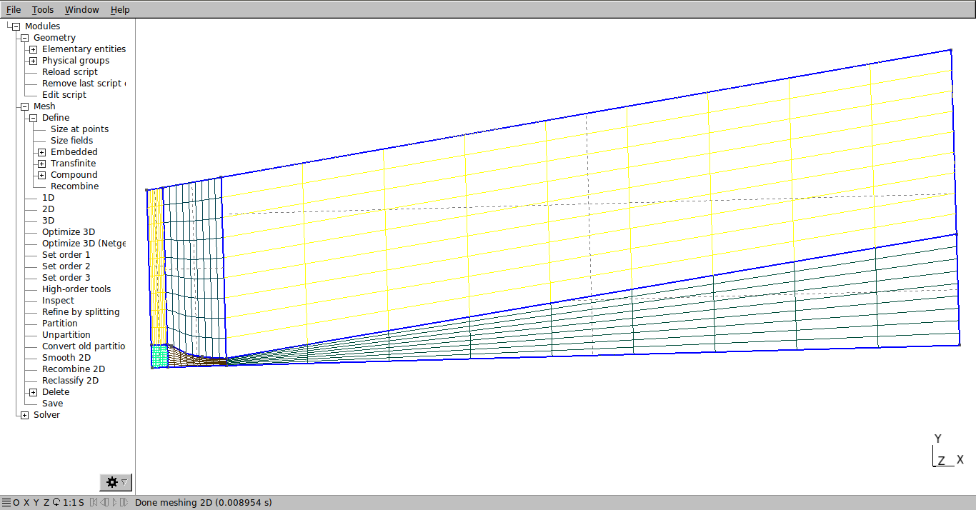
If the mesh is not structured, redo the previous steps.
The values of the function Transfinite must be changed to get the required mesh refinement. First change the variable “a” to 14 and reload the script. Note that the number of volumes at the inlet will increase.
Then change the following variables: b=160 , c= 225, d = 40, e=14, f=160 and g=100.
Now the increase volume rate must be changed to obtain a more refined mesh in certain regions. This is done by changing the variable “Progression” in the Transfinite function. First change the increase rate of the second nozzle division.
\\ internal horizontal lines of the nozzle:

a = 14;
b = 160;
//+
Transfinite Curve {20} = a Using Progression 1;
//+
Transfinite Curve {22} = a Using Progression 1;
//+
Transfinite Curve {26} = b Using Progression 1/1.02;
//+
Transfinite Curve {24} = b Using Progression 1/1.02;
The result should be as shown below.
Note that “1 / 1.02” was written, because the increase rate follows the line direction orientation, as defined in its creation. If the increase rate has been inverted, change to “1.02”. Then, change the increase rate of horizontal lines in front of the nozzle.
// horizontal lines in front of the nozzle:
c = 225;
//+
Transfinite Curve {29} = c Using Progression 1.027;
//+
Transfinite Curve {27} = c Using Progression 1.027;
//+
Transfinite Curve {38} = c Using Progression 1/1.027;
The result should be as following:
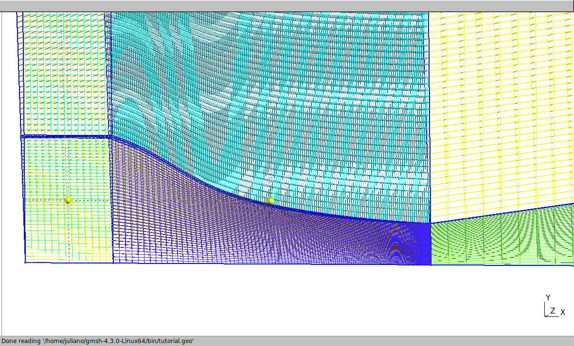
Change the progression of internal vertical lines of the nozzle, in order to increase the refinement of the mesh next to the wall:
// internal vertical lines of the nozzle:
d = 40;
//+
Transfinite Curve {23} = d Using Progression 1.025;
//+
Transfinite Curve {21} = d Using Progression 1/1.015;
//+
Transfinite Curve {25} = d Using Progression 1/1.01;
//+
Transfinite Curve {28} = d Using Progression 1.01;
At the top of the nozzle:
\\external horizontal lines of the nozzle:

e = 14;
f = 160;
//+
Transfinite Curve {31} = e Using Progression 1;
//+
Transfinite Curve {33} = e Using Progression 1;
//+
Transfinite Curve {36} = f Using Progression 1/1.02;
//+
Transfinite Curve {34} = f Using Progression 1.02;

And finally the vertical lines above the nozzle:
// external vertical lines of the nozzle:

g = 100;
//+
Transfinite Curve {30} = g Using Progression 1/1.047;
//+
Transfinite Curve {32} = g Using Progression 1.047;
//+
Transfinite Curve {35} = g Using Progression 1.047;
//+
Transfinite Curve {37} = g Using Progression 1/1.005;

The next step is to extrude the geometry so that it generates the wedge shape. This procedure is required to run the axisymmetric case in OpenFOAM. To do this, go to Modules → Elementary entties → Extrude → Rotate and set the window as shown below.
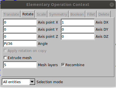
Then, select all the surfaces and press “e” to confirm. The result should be as shown below
To do this process via script, set the following changes to the Extrude function in the .geo file.
// EXTRUSION:
//+
Extrude {{1, 0, 0}, {0, 0, 0}, Pi/36} {
Surface{1}; Surface{2}; Surface{3}; Surface{4}; Surface{5}; Surface{6};
Layers{1};
Recombine;
}
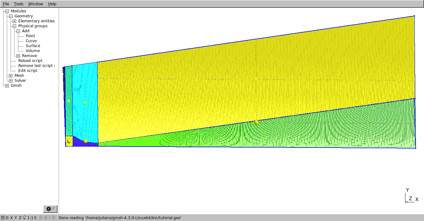
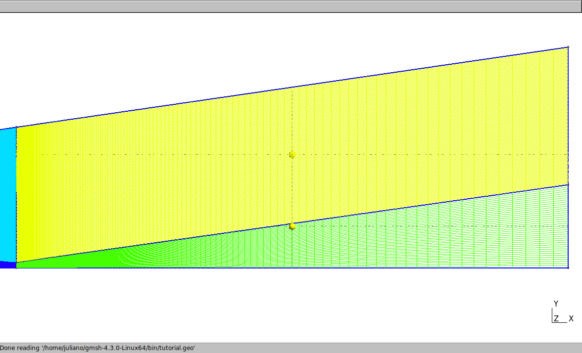
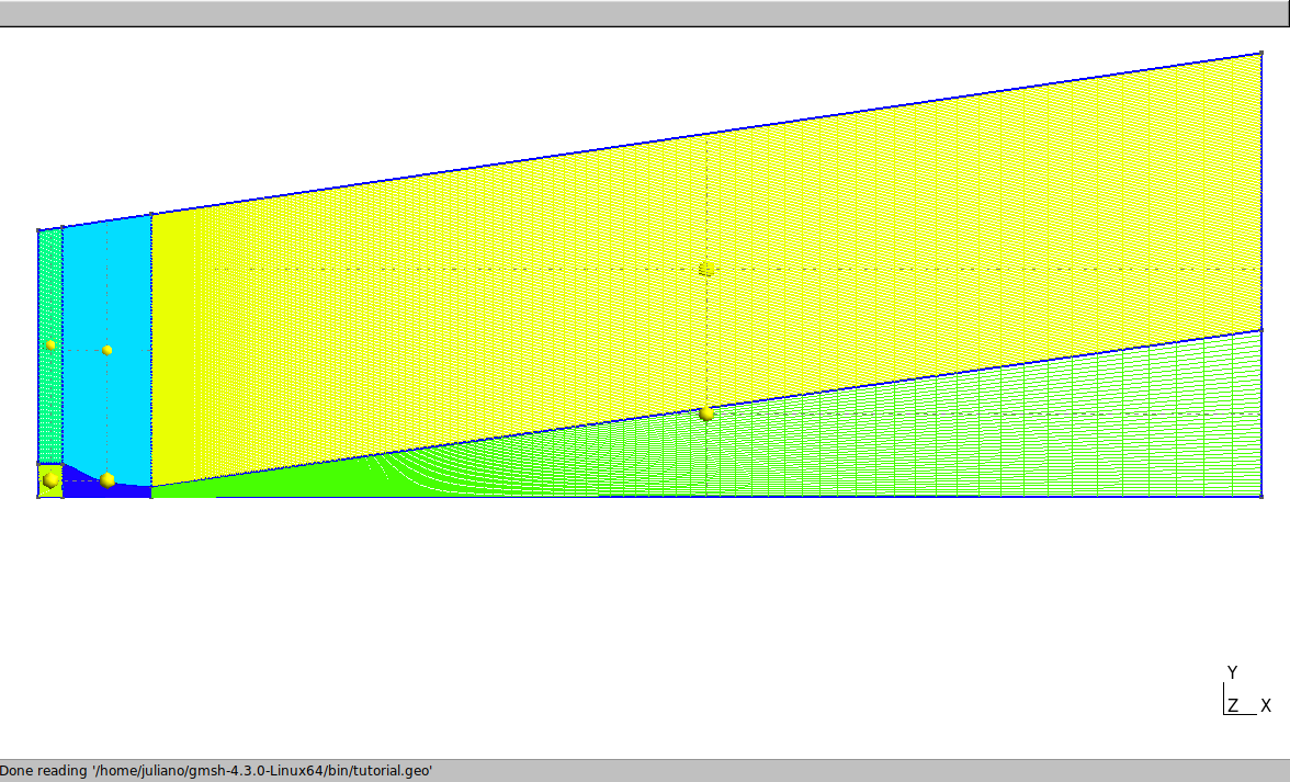
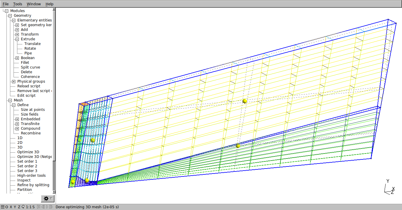
Now it is possible to see the 3D mesh by clicking on Modules → Mesh → 3D. The result should be as shown below. If the mesh has not been structured, review the previous steps.
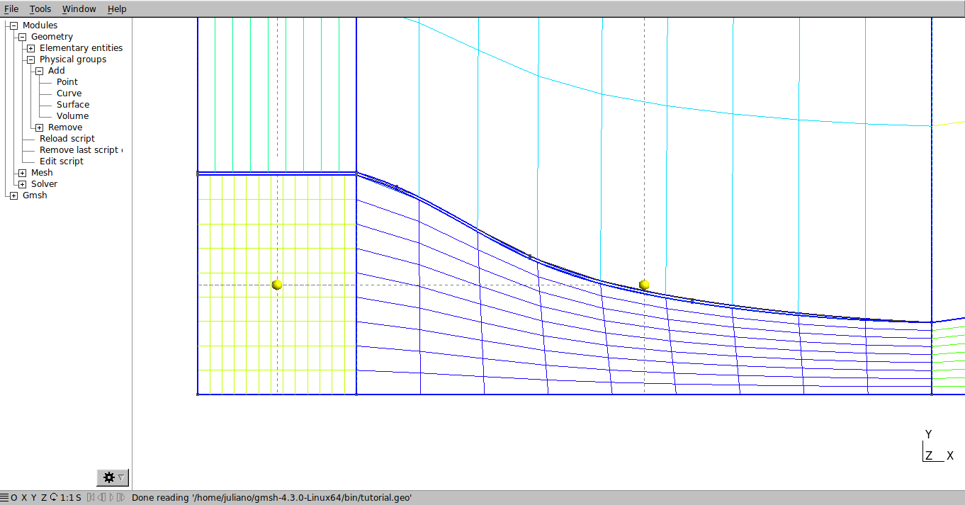
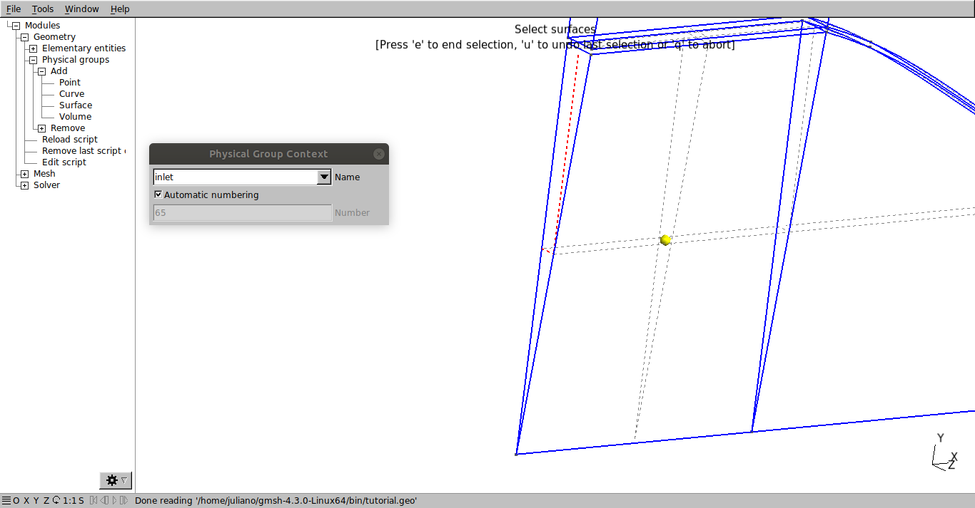
The last step is to define the surface names where the boundary conditions will be set. The names used here will be: inlet, atmosphere, nozzle, wedge_1, wedge_2 and volume. Go to Modules → Geometry → Physical Groups → Add → Surface. Type “inlet”, select the corresponding surface and press “e”.
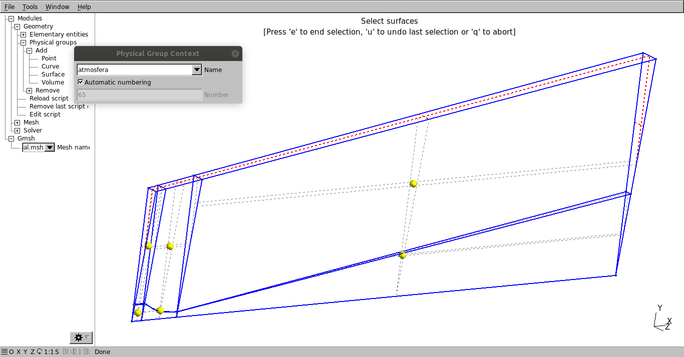
Do the same for the surfaces corresponding to atmosphere, as shown in the figure:
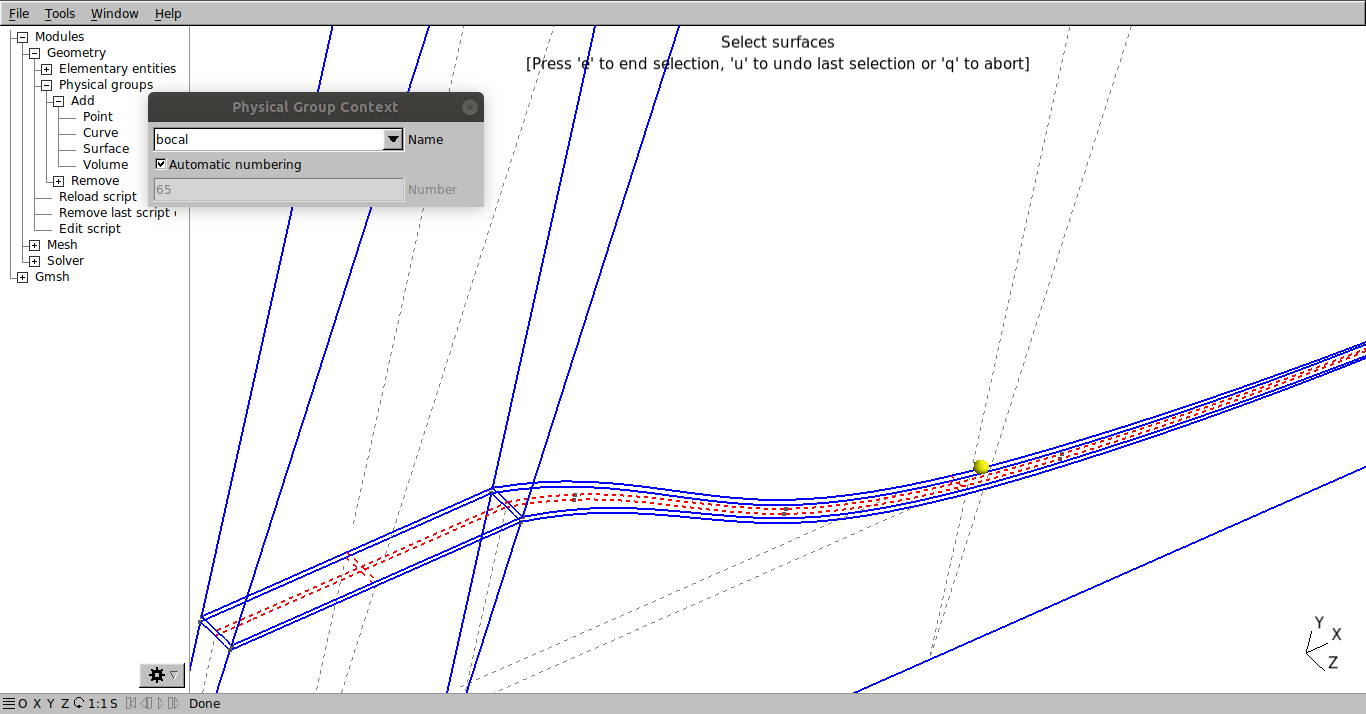
The nozzle:
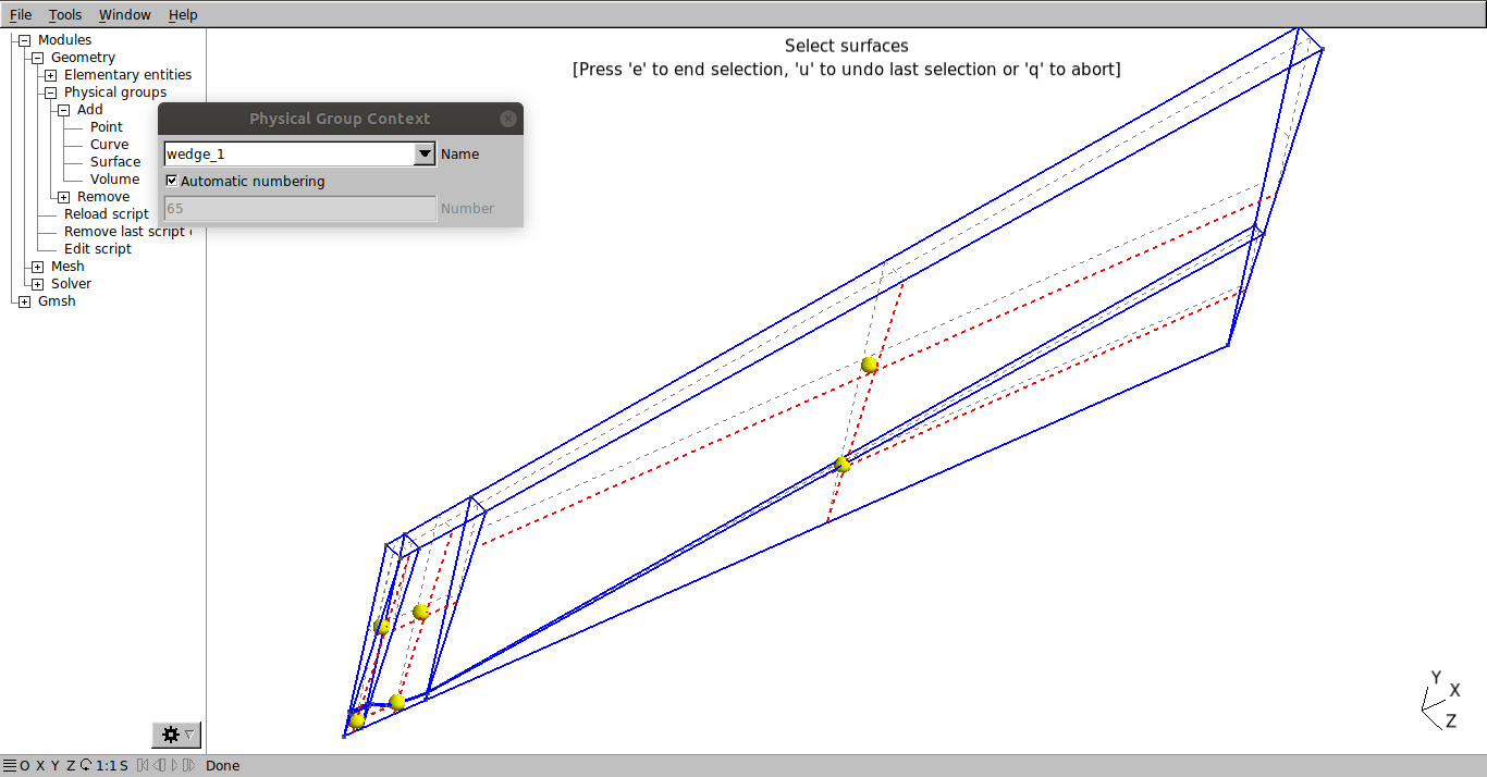
The wedge_1:
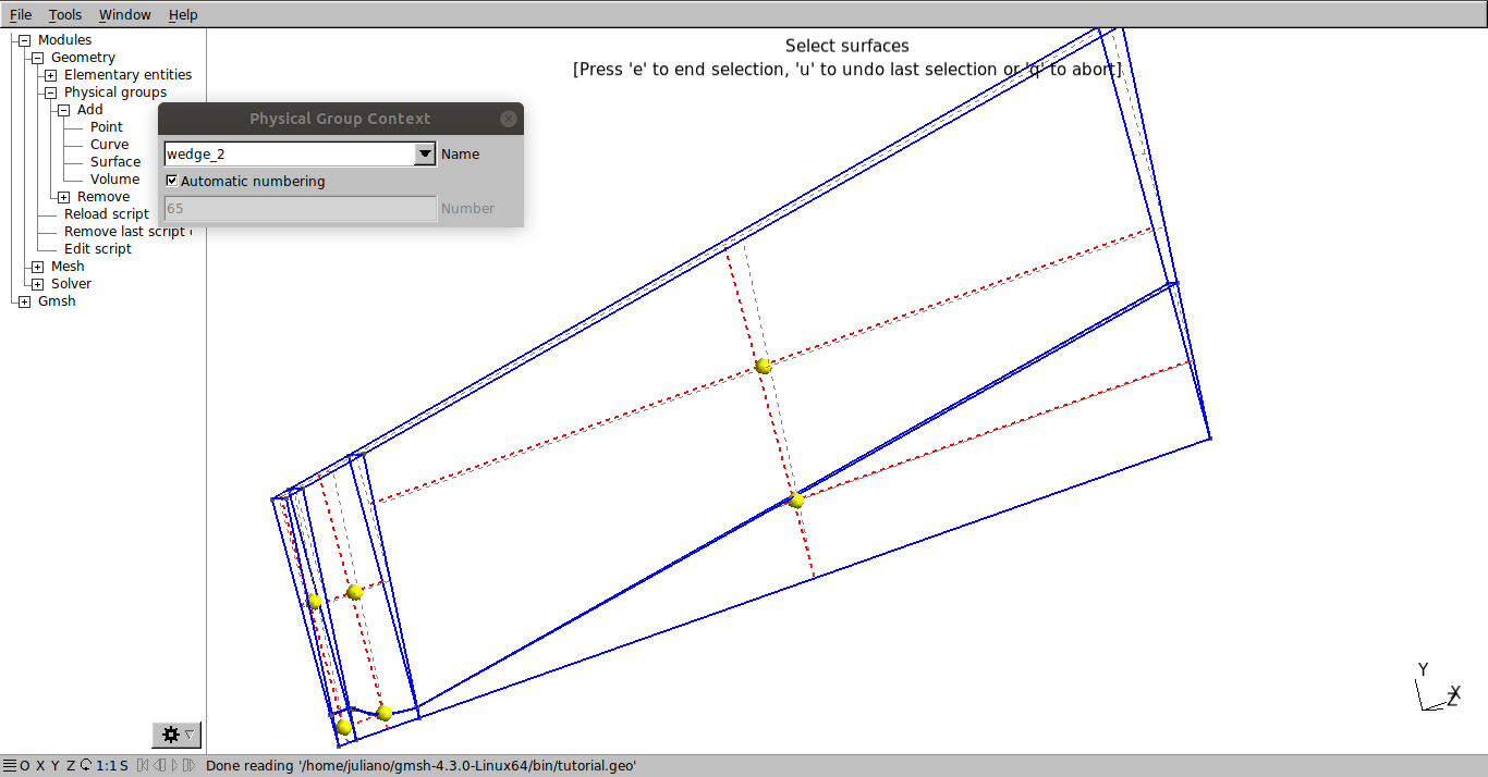
The wedge_2:
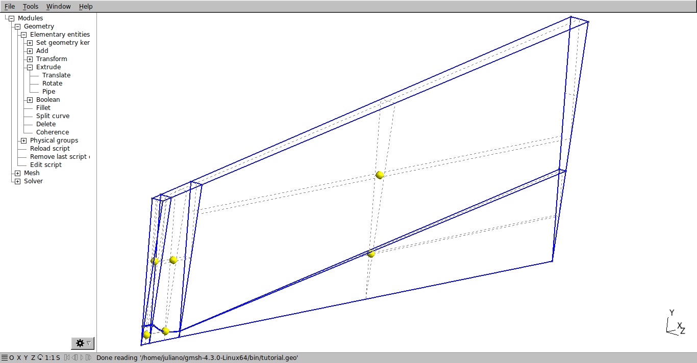
Go to Modules → Geometry → Physical Groups → Add → Volume and select the yellow spheres and press “e” to confirm:
The setting in .geo file should be the following:
//+
Physical Surface("inlet") = {9};
//+
Physical Surface("atmosphera") = {17, 20, 22, 27, 26, 15};
//+
Physical Surface("nozzle") = {18, 24, 11, 8};
//+
Physical Surface("wedge_1") = {10, 13, 16, 21, 25, 28};
//+
Physical Surface("wedge_2") = {1, 2, 3, 4, 5, 6};
//+
Physical Volume("volume") = {1, 2, 3, 4, 5, 6};
Finally , add the command “Mesh 3;” in the .geo file and then the mesh creation is finished. To create the file to be used in OpenFOAM click on File → Export, choose the directory where you want to save it and save with .msh extension. Then, a window showing “MSH Options” will appear, select the format “Version 2 ASCII” and click on save. The output file will be imported in OpenFOAM®.


